Preface: This is the competition of Titanic Machine Learning from Kaggle
The sinking of the RMS Titanic is one of the most infamous shipwrecks in history. On April 15, 1912, during her maiden voyage, the Titanic sank after colliding with an iceberg, killing 1502 out of 2224 passengers and crew. This sensational tragedy shocked the international community and led to better safety regulations for ships.
In this challenge, we ask you to complete the analysis of what sorts of people were likely to survive. In particular, we ask you to apply the tools of machine learning to predict which passengers survived the tragedy.
1. Get the dataset
    train <- read.csv("train.csv")
    test <- read.csv("test.csv")
    library(dplyr)
    full <- bind_rows(train, test)
2. Explore the data
head(full)
##   PassengerId Survived Pclass
## 1           1        0      3
## 2           2        1      1
## 3           3        1      3
## 4           4        1      1
## 5           5        0      3
## 6           6        0      3
##                                                  Name    Sex Age SibSp
## 1                             Braund, Mr. Owen Harris   male  22     1
## 2 Cumings, Mrs. John Bradley (Florence Briggs Thayer) female  38     1
## 3                              Heikkinen, Miss. Laina female  26     0
## 4        Futrelle, Mrs. Jacques Heath (Lily May Peel) female  35     1
## 5                            Allen, Mr. William Henry   male  35     0
## 6                                    Moran, Mr. James   male  NA     0
##   Parch           Ticket    Fare Cabin Embarked
## 1     0        A/5 21171  7.2500              S
## 2     0         PC 17599 71.2833   C85        C
## 3     0 STON/O2. 3101282  7.9250              S
## 4     0           113803 53.1000  C123        S
## 5     0           373450  8.0500              S
## 6     0           330877  8.4583              Q
summary(full)
##   PassengerId      Survived          Pclass          Name
##  Min.   :   1   Min.   :0.0000   Min.   :1.000   Length:1309
##  1st Qu.: 328   1st Qu.:0.0000   1st Qu.:2.000   Class :character
##  Median : 655   Median :0.0000   Median :3.000   Mode  :character
##  Mean   : 655   Mean   :0.3838   Mean   :2.295
##  3rd Qu.: 982   3rd Qu.:1.0000   3rd Qu.:3.000
##  Max.   :1309   Max.   :1.0000   Max.   :3.000
##                 NA's   :418
##      Sex           Age            SibSp            Parch
##  female:466   Min.   : 0.17   Min.   :0.0000   Min.   :0.000
##  male  :843   1st Qu.:21.00   1st Qu.:0.0000   1st Qu.:0.000
##               Median :28.00   Median :0.0000   Median :0.000
##               Mean   :29.88   Mean   :0.4989   Mean   :0.385
##               3rd Qu.:39.00   3rd Qu.:1.0000   3rd Qu.:0.000
##               Max.   :80.00   Max.   :8.0000   Max.   :9.000
##               NA's   :263
##     Ticket               Fare            Cabin
##  Length:1309        Min.   :  0.000   Length:1309
##  Class :character   1st Qu.:  7.896   Class :character
##  Mode  :character   Median : 14.454   Mode  :character
##                     Mean   : 33.295
##                     3rd Qu.: 31.275
##                     Max.   :512.329
##                     NA's   :1
##    Embarked
##  Length:1309
##  Class :character
##  Mode  :character
##
##
##
##
- Survived: 1 is survived, 0 is dead
- Pclass:class level, 1 is first-class, 2 is intermediate, 3 is economy
- Name:name of passenger
- Sex:gender
- Age: age
- SibSp:number of sibling and partner
- Parch:number of parents or children
- Ticket:ticket serial number
- Fare:ticket price
- Cabin:cabin gate
- Embarked:embarked gate
3. Verify the missing number for each variable
sapply(full,function(x) sum(is.na(x)))
## PassengerId    Survived      Pclass        Name         Sex         Age
##           0         418           0           0           0         263
##       SibSp       Parch      Ticket        Fare       Cabin    Embarked
##           0           0           0           1           0           0

sapply(full,function(x) sum(x==''))

## PassengerId    Survived      Pclass        Name         Sex         Age
##           0          NA           0           0           0          NA
##       SibSp       Parch      Ticket        Fare       Cabin    Embarked
##           0           0           0          NA        1014           2
| Variable | Missing data |
|---|---|
| survived | 418 |
| age | 263 |
| fare | 1 |
| Cabin | 1024 |
| Embarked | 2 |
- we can ignore the missing data in “survived” since it is caused by testing data.
- not add missing data in cabin due to lack of methodology
3.1.Add missing data in “Embarked”
    embarked.na <- full$Embarked
    which(embarked.na %in% "")
## [1] 62 830
    #Find out the blank value, we locate 62 and 830
    full_62 <- full[full$PassengerId==62,]
    full_62
##    PassengerId Survived Pclass                Name    Sex Age SibSp Parch
## 62          62        1      1 Icard, Miss. Amelie female  38     0     0
##    Ticket Fare Cabin Embarked
## 62 113572   80   B28
    full_830 <- full[full$PassengerId==830,]
    full_830
##     PassengerId Survived Pclass                                      Name
## 830         830        1      1 Stone, Mrs. George Nelson (Martha Evelyn)
##        Sex Age SibSp Parch Ticket Fare Cabin Embarked
## 830 female  62     0     0 113572   80   B28
    library(ggplot2)
    library(scales)
    library(ggthemes)
    embark_fare <- full %>% filter(PassengerId !=62 & PassengerId !=830)
    ggplot(embark_fare, aes(x=Embarked, y=Fare, fill=factor(Pclass)))+geom_boxplot()+geom_hline(aes(yintercept=80), colour='red', linetype='dashed',lwd=2)+scale_y_continuous(labels=dollar_format())+theme_few()+ggtitle('the embarkment by passenger class and median fare')
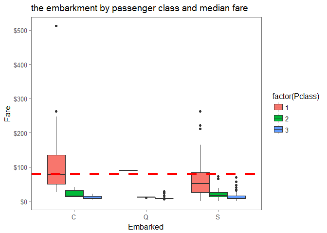
add “C” to blank value
    full$Embarked[c(62, 830)] <- 'C'
    sapply(full,function(x) sum(x==''))
## PassengerId    Survived      Pclass        Name         Sex         Age
##           0          NA           0           0           0          NA
##       SibSp       Parch      Ticket        Fare       Cabin    Embarked
##           0           0           0          NA        1014           0
3.2 Add missing data in “Fare”
    Fare.na <- is.na(full$Fare)
    which(Fare.na %in% TRUE)
## [1] 1044
full[1044,]
##      PassengerId Survived Pclass               Name  Sex  Age SibSp Parch
## 1044        1044       NA      3 Storey, Mr. Thomas male 60.5     0     0
##      Ticket Fare Cabin Embarked
## 1044   3701   NA              S
    full_fare <- full[full$Pclass=='3'&full$Embarked=='S', ]

    ggplot(full_fare, aes(x=Fare))+geom_density(fill='skyblue',alpha=0.4)+geom_vline(aes(xintercept=median(Fare,na.rm=T)), colour='red', linetype='dashed',lwd=1)+scale_y_continuous(labels=dollar_format())+theme_few()+ggtitle('the density of Fare')
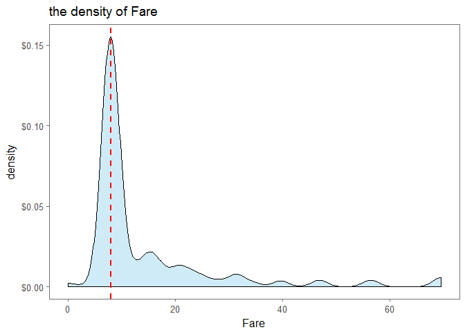
we can conclude that the passenger embarked at S and Pclass=3 paid $0-20. Then we can add the missing value with median
full$Fare[1044] = median(full_fare$Fare, na.rm=T)
3.3 Add missing data in “Age”
    set.seed(123)
    library(mice)

    #delete the variables that are not necessary
    A <- c('PassengerId','Name','Ticket','Cabin','family','Surname','Survived')
    mice_mod <- mice(full[,!names(full) %in% A],method = 'rf')
##
##  iter imp variable
##   1   1  Age
##   1   2  Age
##   1   3  Age
##   1   4  Age
##   1   5  Age
##   2   1  Age
##   2   2  Age
##   2   3  Age
##   2   4  Age
##   2   5  Age
##   3   1  Age
##   3   2  Age
##   3   3  Age
##   3   4  Age
##   3   5  Age
##   4   1  Age
##   4   2  Age
##   4   3  Age
##   4   4  Age
##   4   5  Age
##   5   1  Age
##   5   2  Age
##   5   3  Age
##   5   4  Age
##   5   5  Age
mice_output <- complete(mice_mod)
compare the forecasting by MICE with original data
    par(mfrow=c(1,2))
    hist(full$Age,freq = F,main = 'Age:ORiginal Data',col='darkblue',ylim = c(0,0.04))
    hist(mice_output$Age,freq = F,main = 'Age:MICE Output',col = 'skyblue',ylim = c(0,0.04))
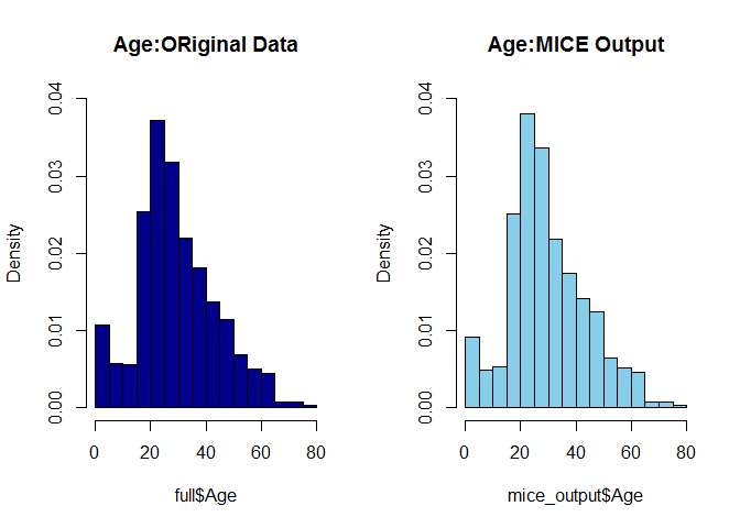
We can use forecast to fill up the missing data since both are similar
full$Age <- mice_output$Age
make sure there are no missing data
sum(is.na(full$Age))
## [1] 0
sum(is.na(full$Fare))
## [1] 0
3.4 drop Cabin variable
    drops <- c("Cabin")
    full = full[ , !(names(full) %in% drops)]
let us take a look at the final version of dataset
summary(full)
##   PassengerId      Survived          Pclass          Name
##  Min.   :   1   Min.   :0.0000   Min.   :1.000   Length:1309
##  1st Qu.: 328   1st Qu.:0.0000   1st Qu.:2.000   Class :character
##  Median : 655   Median :0.0000   Median :3.000   Mode  :character
##  Mean   : 655   Mean   :0.3838   Mean   :2.295
##  3rd Qu.: 982   3rd Qu.:1.0000   3rd Qu.:3.000
##  Max.   :1309   Max.   :1.0000   Max.   :3.000
##                 NA's   :418
##      Sex           Age            SibSp            Parch
##  female:466   Min.   : 0.17   Min.   :0.0000   Min.   :0.000
##  male  :843   1st Qu.:21.00   1st Qu.:0.0000   1st Qu.:0.000
##               Median :28.00   Median :0.0000   Median :0.000
##               Mean   :30.25   Mean   :0.4989   Mean   :0.385
##               3rd Qu.:39.00   3rd Qu.:1.0000   3rd Qu.:0.000
##               Max.   :80.00   Max.   :8.0000   Max.   :9.000
##
##     Ticket               Fare           Embarked
##  Length:1309        Min.   :  0.000   Length:1309
##  Class :character   1st Qu.:  7.896   Class :character
##  Mode  :character   Median : 14.454   Mode  :character
##                     Mean   : 33.276
##                     3rd Qu.: 31.275
##                     Max.   :512.329
##
4 Analyze the dataset
4.1 how title realtes with survival rate.
    library(stringr)
    #fecth the title
    full$Title <- gsub('(.*, )|(\\..*)','',full$Name)

    #check the category of name
    table(full$Sex, full$Title)
##
##          Capt Col Don Dona  Dr Jonkheer Lady Major Master Miss Mlle Mme
##   female    0   0   0    1   1        0    1     0      0  260    2   1
##   male      1   4   1    0   7        1    0     2     61    0    0   0
##
##           Mr Mrs  Ms Rev Sir the Countess
##   female   0 197   2   0   0            1
##   male   757   0   0   8   1            0
    #combine the rare
    rare_title <- c('Capt','Col','Don','Dona','Dr','Jonkheer','Lady','Major','Rev','Sir','the Countess')

    #regulate the title
    full$Title[full$Title=='Mlle'] <- 'Miss'
    full$Title[full$Title=='Mme'] <- 'Mrs'
    full$Title[full$Title=='Ms'] <- 'Miss'
    full$Title[full$Title %in% rare_title] <- 'Rare title'

    summary(full)
##   PassengerId      Survived          Pclass          Name
##  Min.   :   1   Min.   :0.0000   Min.   :1.000   Length:1309
##  1st Qu.: 328   1st Qu.:0.0000   1st Qu.:2.000   Class :character
##  Median : 655   Median :0.0000   Median :3.000   Mode  :character
##  Mean   : 655   Mean   :0.3838   Mean   :2.295
##  3rd Qu.: 982   3rd Qu.:1.0000   3rd Qu.:3.000
##  Max.   :1309   Max.   :1.0000   Max.   :3.000
##                 NA's   :418
##      Sex           Age            SibSp            Parch
##  female:466   Min.   : 0.17   Min.   :0.0000   Min.   :0.000
##  male  :843   1st Qu.:21.00   1st Qu.:0.0000   1st Qu.:0.000
##               Median :28.00   Median :0.0000   Median :0.000
##               Mean   :30.25   Mean   :0.4989   Mean   :0.385
##               3rd Qu.:39.00   3rd Qu.:1.0000   3rd Qu.:0.000
##               Max.   :80.00   Max.   :8.0000   Max.   :9.000
##
##     Ticket               Fare           Embarked
##  Length:1309        Min.   :  0.000   Length:1309
##  Class :character   1st Qu.:  7.896   Class :character
##  Mode  :character   Median : 14.454   Mode  :character
##                     Mean   : 33.276
##                     3rd Qu.: 31.275
##                     Max.   :512.329
##
##     Title
##  Length:1309
##  Class :character
##  Mode  :character
##
##
##
##
    #check the category of name
    table(full$Sex, full$Title)
##
##          Master Miss  Mr Mrs Rare title
##   female      0  264   0 198          4
##   male       61    0 757   0         25
compare the variables
    library(ggplot2)
    ggplot(full[1:891,], aes(Title, fill=factor(Survived)))+geom_bar()+facet_grid(.~Sex)+theme_few()+ggtitle('The Survival by Title and Sex')
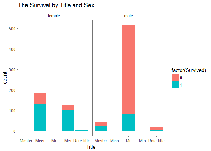
Obviously, “Miss”, “Mrs” has significant survival rate. “Mr” has significant mortality
4.2 how sex realtes with survival rate.
mosaicplot(table(full$Sex, full$Survived), main='survival by Sex', shade=T)
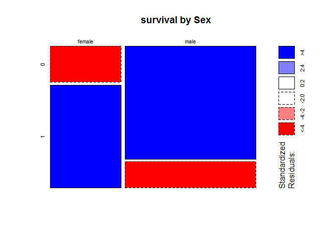
Female has higher survival rate, but how about rate for those who are mother?
    full$mother <- 'not mother'
    full$mother[full$Sex == 'female' & full$Age>18 & full$Parch>0 & full$Title !='Miss'] <- 'mother'
    mosaicplot(table(full$mother, full$Survived), main='survival by mother', color=c('skyblue','pink'))
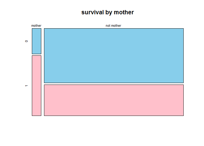
mother has higher survival rate
4.3 how family member affects the survival rate
    full$familysize <- full$SibSp+full$Parch+1

    #fecth family name
    full$Surname <- sapply(strsplit(full$Name,split = '[,.]'),'[',1)
    ggplot(full[1:891,],aes(x=familysize,fill=factor(Survived)))+geom_bar(stat = 'count',position='dodge')+scale_x_continuous(breaks = c(1:11))+labs(x='Family size')+theme_bw()+ggtitle("Family size VS Survived")
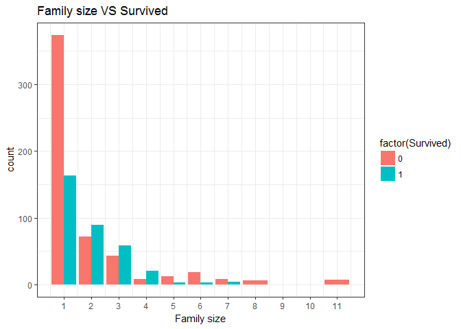
higher survival rate for the family size 1-4
categorize the family into bachelor, small and big
    full$Fsize[full$familysize==1] <- 'singleton'
    full$Fsize[full$familysize>1&full$familysize<5] <- 'small family'
    full$Fsize[full$familysize>=5] <- 'big family'

    mosaicplot(table(full$Fsize,full$Survived),main = 'Family Size by Survival',shade = T)
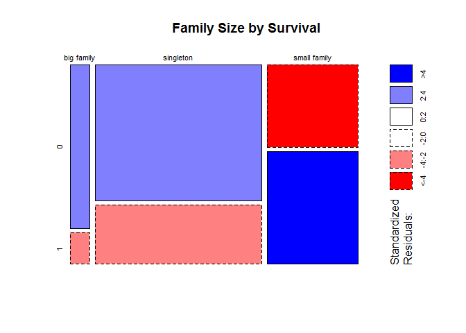
small family has higher survival rate
4.4 how age affects the survival rate
ggplot(full[1:891,],aes(Age,fill=factor(Survived)))+geom_histogram()+facet_grid(.~Sex)+theme_few()+ggtitle('The Survival by Age and Sex')
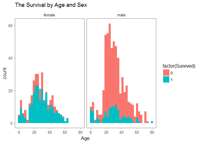
age 0-20 has higher survival rate regardless of gender
categorize age into child and adult
    full$child[full$Age < 18] <- 'child'
    full$child[full$Age >= 18] <- 'adult'
    table(full$child,full$Survived)
##
##           0   1
##   adult 489 275
##   child  60  67
mosaicplot(table(full$child,full$Survived),main = 'The Survival by Age',shade = T)
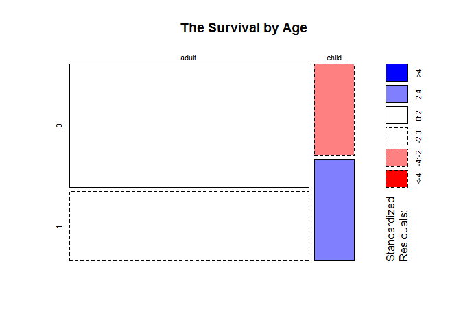
children has higher survival rate than adult
4.5 how ticket price affects the survival rate
categorize price into low, middle, high
    full$Fare1 = "low"
    full$Fare1[full$Fare>=100 & full$Fare <=300] = 'middle'
    full$Fare1[full$Fare>300] = 'high'

    mosaicplot(table(full$Fare1,full$Survived),main = 'The Survival by Ticket price',shade = T)
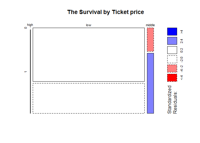
cheap ticket has lower survival rate. Cross check with the below
    rate_survived <- function(n){
      full_rate <- xtabs(~n+Survived,data = full)
      rate <- prop.table(full_rate,1)
      return(rate)
    }
    rate_survived(full$Fare1)
##         Survived
## n                0         1
##   high   0.0000000 1.0000000
##   low    0.6384248 0.3615752
##   middle 0.2800000 0.7200000
5 Model Building
5.1 In the analysis in section 4, we consider Pclass+Fare+Embarked+Title++Sex+Fsize+child
    train <- full[1:891,]
    test <- full[892:1309,]
    #to avoid error msg of NA enforced in randomForest
    train$Embarked = as.factor(train$Embarked)
    train$Title = as.factor(train$Title)
    train$Fsize = as.factor(train$Fsize)
    train$child = as.factor(train$child)

    test$Embarked = as.factor(test$Embarked)
    test$Title = as.factor(test$Title)
    test$Fsize = as.factor(test$Fsize)
    test$child = as.factor(test$child)
    library(randomForest)
    set.seed(754)

    rf_mode <- randomForest(factor(Survived)~Pclass+Fare+Embarked+Title+Sex+Fsize+child,data = train)

    plot(rf_mode,ylim = c(0,0.36))
    legend('topright',colnames(rf_mode$err.rate),col=1:3,fill=1:3)
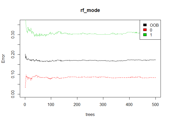
error rate of mortality is 0.1, error rate of survival is 0.3. It means it it much easier to determine if the passenger is dead.
5.2 analyze on the weigh of factor
    #fetch important factors
    importance <- importance(rf_mode)
    varImportance <- data.frame(variables=row.names(importance),Importance=round(importance[,'MeanDecreaseGini'],2))
    ###sort the variable by factors
    library(dplyr)
    rankImportance <- varImportance %>% mutate(Ranke=paste0('#',dense_rank(desc(Importance))))

    ggplot(rankImportance,aes(x=reorder(variables,Importance),y=Importance,fill=Importance))+   geom_bar(stat='identity')+  geom_text(aes(x=variables,y=0.5,label=Ranke),hjust=0,vjust=0.55,size=4,colour='red')+   labs(x='Variables')+   coord_flip()+theme_few()+ggtitle('The Importance of Variables')
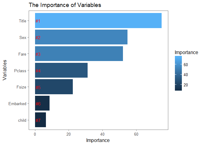
the top 3 important factors are Title, Sex, Fare
Predict
    prediction <- predict(rf_mode,test)

    solution <- data.frame(PassengerId=test$PassengerId,Survived=prediction)

    # write.csv(solution,file='solution',row.names=F)