Lazy Learning - Classification Using Nearest Neighbors

Understanding classification using nearest neighbors

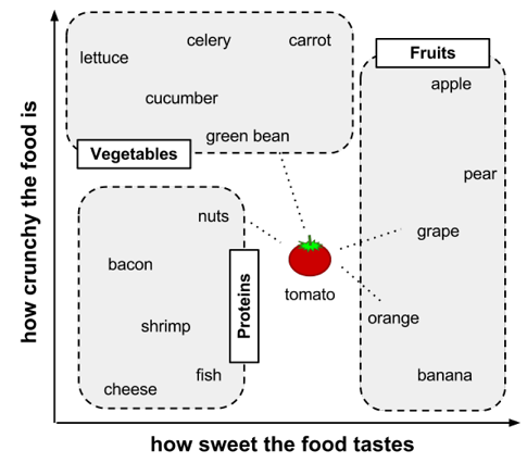
Define feature, link your train example (food) to the result (food type)
Treat the features as coordinates in a multidimensional feature space
Notice pattern (Similar types of food tend to be grouped closely together)
Use a nearest neighbor approach to determine which class is a better fit the test example
Calculate distance
- Euclidean distance is measured “as the crow flies,” implying the shortest direct route. Euclidean distance is specified by the following formula. The term p1 refers to the value of the first feature of example p, while q1 refers to the value of the first feature of example q: $dist(P,Q) = \\sqrt{(P\_1 - Q\_1)^2 + (P\_2 - Q\_2)^2 + ... + (P\_n - Q\_n)^2}$
- Another common distance measure is Manhattan distance, which is based on the paths a pedestrian would take by walking city blocks.
Use KNN algorithm to determine which category it belongs to:

ingredient	sweetness	crunchiness	food type	distance to the tomato
grape	8	5	fruit	sqrt((6 - 8)^2 + (4 - 5)^2) = 2.2
green bean	3	7	vegetable	sqrt((6 - 3)^2 + (4 - 7)^2) = 4.2
nuts	3	6	protein	sqrt((6 - 3)^2 + (4 - 6)^2) = 3.6
orange	7	3	fruit	sqrt((6 - 7)^2 + (4 - 3)^2) = 1.4

If K = 1, the orange is the nearest neighbor to the tomato, with a distance of 1.4. As orange is a fruit, the 1NN algorithm would classify tomato as a fruit.
If K = 3, it performs a vote among the three nearest neighbors: orange, grape, and nuts. Because the majority class among these neighbors is fruit (2 of the 3 votes), the tomato again is classified as a fruit.

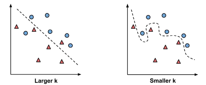
Choosing an appropriate k: The following figure illustrates more generally how the decision boundary (depicted by a dashed line) is affected by larger or smaller k values. Smaller values allow more complex decision boundaries that more carefully fit the training data. The problem is that we do not know whether the straight boundary or the curved boundary better represents the true underlying concept to be learned.

One common practice is to set k equal to the square root of the number of training examples. An alternative approach is to test several k values on a variety of test datasets and choose the one that delivers the best classification performance - Choosing a large k reduces the impact or variance caused by noisy data, but can bias the learner such that it runs the risk of ignoring small, but important patterns. - Using a single nearest neighbor allows noisy data or outliers, to unduly influence the classification of examples.

What we need is a way of “shrinking” or rescaling the various features such that each one contributes relatively equally to the distance formula.

The traditional method of rescaling features for kNN is min-max normalization. Normalized feature values can be interpreted as indicating how far, from 0 percent to 100 percent, the original value fell along the range between the original minimum and maximum $X\_{new} = \\frac{X-Min(X)}{Max(X)-Min(X)}$
Another common transformation is called z-score standardization $X\_{new} = \\frac{X-Mean(X)}{StdDev(X)}$
Dummy coding The Euclidean distance formula is not defined for nominal data. Therefore, to calculate the distance between nominal features, we need to convert them into a numeric format. A typical solution utilizes dummy coding, where a value of 1 indicates one category, and 0 indicates the other

Diagnosing breast cancer with the kNN algorithm

We will investigate the utility of machine learning for detecting cancer by applying the kNN algorithm to measurements of biopsied cells from women with abnormal breast masses.

Step 1 - collecting data

wbcd <- read.csv("wisc_bc_data.csv", stringsAsFactors = FALSE)

Step 2 - exploring and preparing the data

str(wbcd)

## 'data.frame':    569 obs. of  32 variables:
##  $ id               : int  87139402 8910251 905520 868871 9012568 906539 925291 87880 862989 89827 ...
##  $ diagnosis        : chr  "B" "B" "B" "B" ...
##  $ radius_mean      : num  12.3 10.6 11 11.3 15.2 ...
##  $ texture_mean     : num  12.4 18.9 16.8 13.4 13.2 ...
##  $ perimeter_mean   : num  78.8 69.3 70.9 73 97.7 ...
##  $ area_mean        : num  464 346 373 385 712 ...
##  $ smoothness_mean  : num  0.1028 0.0969 0.1077 0.1164 0.0796 ...
##  $ compactness_mean : num  0.0698 0.1147 0.078 0.1136 0.0693 ...
##  $ concavity_mean   : num  0.0399 0.0639 0.0305 0.0464 0.0339 ...
##  $ points_mean      : num  0.037 0.0264 0.0248 0.048 0.0266 ...
##  $ symmetry_mean    : num  0.196 0.192 0.171 0.177 0.172 ...
##  $ dimension_mean   : num  0.0595 0.0649 0.0634 0.0607 0.0554 ...
##  $ radius_se        : num  0.236 0.451 0.197 0.338 0.178 ...
##  $ texture_se       : num  0.666 1.197 1.387 1.343 0.412 ...
##  $ perimeter_se     : num  1.67 3.43 1.34 1.85 1.34 ...
##  $ area_se          : num  17.4 27.1 13.5 26.3 17.7 ...
##  $ smoothness_se    : num  0.00805 0.00747 0.00516 0.01127 0.00501 ...
##  $ compactness_se   : num  0.0118 0.03581 0.00936 0.03498 0.01485 ...
##  $ concavity_se     : num  0.0168 0.0335 0.0106 0.0219 0.0155 ...
##  $ points_se        : num  0.01241 0.01365 0.00748 0.01965 0.00915 ...
##  $ symmetry_se      : num  0.0192 0.035 0.0172 0.0158 0.0165 ...
##  $ dimension_se     : num  0.00225 0.00332 0.0022 0.00344 0.00177 ...
##  $ radius_worst     : num  13.5 11.9 12.4 11.9 16.2 ...
##  $ texture_worst    : num  15.6 22.9 26.4 15.8 15.7 ...
##  $ perimeter_worst  : num  87 78.3 79.9 76.5 104.5 ...
##  $ area_worst       : num  549 425 471 434 819 ...
##  $ smoothness_worst : num  0.139 0.121 0.137 0.137 0.113 ...
##  $ compactness_worst: num  0.127 0.252 0.148 0.182 0.174 ...
##  $ concavity_worst  : num  0.1242 0.1916 0.1067 0.0867 0.1362 ...
##  $ points_worst     : num  0.0939 0.0793 0.0743 0.0861 0.0818 ...
##  $ symmetry_worst   : num  0.283 0.294 0.3 0.21 0.249 ...
##  $ dimension_worst  : num  0.0677 0.0759 0.0788 0.0678 0.0677 ...

The breast cancer data includes 569 examples of cancer biopsies, each with 32 features.
One feature is an identification number, another is the cancer diagnosis, and 30 are numeric-valued laboratory measurements.
The diagnosis is coded as M to indicate malignant or B to indicate benign.

Regardless of the machine learning method, ID variables should always be excluded. Neglecting to do so can lead to erroneous findings because the ID can be used to uniquely “predict” each example. Therefore, a model that includes an identifier will most likely suffer from overfitting, and is not likely to generalize well to other data.

# drop the id feature altogether
wbcd <- wbcd[-1]

The next variable, diagnosis, is of particular interest, as it is the outcome we hope to predict.

table(wbcd$diagnosis)

## 
##   B   M 
## 357 212

The table() output indicates that 357 masses are benign while 212 are malignant:

Many R machine learning classifiers require that the target feature is coded as a factor, so we will need to recode the diagnosis variable. We will also take this opportunity to give the B and M values more informative labels using the labels parameter:

wbcd$diagnosis <- factor(wbcd$diagnosis, levels = c("B", "M"), labels = c("Benign", "Malignant"))
round(prop.table(table(wbcd$diagnosis)) * 100, digits = 1)

## 
##    Benign Malignant 
##      62.7      37.3

The values have been labeled Benign and Malignant, with 62.7 percent and 37.3 percent of the masses, respectively

summary(wbcd[c("radius_mean", "area_mean", "smoothness_mean")])

##   radius_mean       area_mean      smoothness_mean  
##  Min.   : 6.981   Min.   : 143.5   Min.   :0.05263  
##  1st Qu.:11.700   1st Qu.: 420.3   1st Qu.:0.08637  
##  Median :13.370   Median : 551.1   Median :0.09587  
##  Mean   :14.127   Mean   : 654.9   Mean   :0.09636  
##  3rd Qu.:15.780   3rd Qu.: 782.7   3rd Qu.:0.10530  
##  Max.   :28.110   Max.   :2501.0   Max.   :0.16340

The distance calculation for kNN is heavily dependent upon the measurement scale of the input features. As smoothness_mean ranges from 0.05 to 0.16, while area_mean ranges from 143.5 to 2501.0, the impact of area is going to be much larger than smoothness in the distance calculation. This could potentially cause problems for our classifier, so let’s apply normalization to rescale the features to a standard range of values.

Transformation - normalizing numeric data

To normalize these features, we need to create a normalize() function in R. This function takes a vector x of numeric values, and for each value in x, subtract the minimum value in x and divide by the range of values in x. Finally, the resulting vector is returned.

normalize <- function(x) {
  return ((x-min(x)) / (max(x) - min(x)))
}
# test normalize function
normalize(c(1, 2, 3, 4, 5))

## [1] 0.00 0.25 0.50 0.75 1.00

normalize(c(10, 20, 30, 40, 50))

## [1] 0.00 0.25 0.50 0.75 1.00

Despite the fact that the values in the second vector are 10 times larger than the first vector, after normalization, they both appear exactly the same.

Rather than normalizing each of the 30 numeric variables individually, we will use one of R’s functions to automate the process.

wbcd_n <- as.data.frame(lapply(wbcd[2:31], normalize))

This command applies the normalize() function to columns 2 through 31 in the wbcd data frame, converts the resulting list to a data frame, and assigns it the name wbcd_n. The _n suffix is used here as a reminder that the values in wbcd have been normalized.

summary(wbcd_n$area_mean)

##    Min. 1st Qu.  Median    Mean 3rd Qu.    Max. 
##  0.0000  0.1174  0.1729  0.2169  0.2711  1.0000

As expected, the area_mean variable, which originally ranged from 143.5 to 2501.0, now ranges from 0 to 1.

Data preparation - creating training and test datasets

We can simulate this scenario by dividing our data into two portions: a training dataset that will be used to build the kNN model and a test dataset that will be used to estimate the predictive accuracy of the model.

wbcd_train <- wbcd_n[1:469, ]
wbcd_test <- wbcd_n[470:569, ]

In the case that we just saw, the records were already sorted in a random order, so we could simply extract 100 consecutive records to create a test dataset. This would not be an appropriate method if the data was ordered in a non-random pattern such as chronologically, or in groups of similar values. In these cases, random sampling methods would be needed.

When we constructed our training and test data, we excluded the target variable, diagnosis. For training the kNN model, we will need to store these class labels in factor vectors, divided to the training and test datasets:

wbcd_train_labels <- wbcd[1:469, 1]
wbcd_test_labels <- wbcd[470:569, 1]

Step 3 - training a model on the data

For the kNN algorithm, the training phase actually involves no model building–the process of training a lazy learner like kNN simply involves storing the input data in a structured format.

library(class)

# knn Grammer, the function returns a factor vector of predicted  classes for each row in the test data frame.
p <- knn(train, test, class, k)

As our training data includes 469 instances, we might try k = 21, an odd number roughly equal to the square root of 469. Using an odd number will reduce the chance of ending with a tie vote.

wbcd_test_pred <- knn(train = wbcd_train, test = wbcd_test, cl = wbcd_train_labels, k = 21)
wbcd_test_pred

##   [1] Benign    Benign    Benign    Benign    Malignant Benign    Malignant
##   [8] Benign    Malignant Benign    Malignant Benign    Malignant Malignant
##  [15] Benign    Benign    Malignant Benign    Malignant Benign    Malignant
##  [22] Malignant Malignant Malignant Benign    Benign    Benign    Benign   
##  [29] Malignant Malignant Malignant Benign    Malignant Malignant Benign   
##  [36] Benign    Benign    Benign    Benign    Malignant Malignant Benign   
##  [43] Malignant Malignant Benign    Malignant Malignant Malignant Malignant
##  [50] Malignant Benign    Benign    Benign    Benign    Benign    Benign   
##  [57] Benign    Benign    Malignant Benign    Benign    Benign    Benign   
##  [64] Benign    Malignant Malignant Benign    Benign    Benign    Benign   
##  [71] Benign    Malignant Benign    Benign    Malignant Malignant Benign   
##  [78] Benign    Benign    Benign    Benign    Benign    Benign    Malignant
##  [85] Benign    Benign    Malignant Benign    Benign    Benign    Benign   
##  [92] Malignant Benign    Benign    Benign    Benign    Benign    Malignant
##  [99] Benign    Malignant
## Levels: Benign Malignant

Step 4 - evaluating model performance

The next step of the process is to evaluate how well the predicted classes in the wbcd_test_pred vector match up with the known values in the wbcd_test_labels vector.

library(gmodels)

## Warning: package 'gmodels' was built under R version 3.3.3

CrossTable(x = wbcd_test_labels, y = wbcd_test_pred, prop.chisq = FALSE)

## 
##  
##    Cell Contents
## |-------------------------|
## |                       N |
## |           N / Row Total |
## |           N / Col Total |
## |         N / Table Total |
## |-------------------------|
## 
##  
## Total Observations in Table:  100 
## 
##  
##                  | wbcd_test_pred 
## wbcd_test_labels |    Benign | Malignant | Row Total | 
## -----------------|-----------|-----------|-----------|
##           Benign |        61 |         0 |        61 | 
##                  |     1.000 |     0.000 |     0.610 | 
##                  |     0.968 |     0.000 |           | 
##                  |     0.610 |     0.000 |           | 
## -----------------|-----------|-----------|-----------|
##        Malignant |         2 |        37 |        39 | 
##                  |     0.051 |     0.949 |     0.390 | 
##                  |     0.032 |     1.000 |           | 
##                  |     0.020 |     0.370 |           | 
## -----------------|-----------|-----------|-----------|
##     Column Total |        63 |        37 |       100 | 
##                  |     0.630 |     0.370 |           | 
## -----------------|-----------|-----------|-----------|
## 
## 

In the top-left cell (labeled TN), are the true negative results. These 61 of 100 values indicate cases where the mass was benign, and the kNN algorithm correctly identified it as such
The bottom-right cell (labeled TP), indicates the true positive results, where the classifier and the clinically determined label agree that the mass is malignant. A total of 37 of 100 predictions were true positives.
The 2 examples in the lower-left FN cell are false negative results; in this case, the predicted value was benign but the tumor was actually malignant. Errors in this direction could be extremely costly, as they might lead a patient to believe that she is cancer-free, when in reality the disease may continue to spread.
The cell labeled FP would contain the false positive results,if there were any. These values occur when the model classifies a mass as malignant when in reality it was benign. Although such errors are less dangerous than a false negative result, they should also be avoided as they could lead to additional financial burden on the health care system, or additional stress for the patient, as additional tests or treatment may have to be provided.

Step 5 - improving model performance

First, we will employ an alternative method for rescaling our numeric features. Second, we will try several different values for k.

Transformation - z-score standardization

The scale() function offers the additional benefit that it can be applied directly to a data frame, so we can avoid use of the lapply() function.

# Rescales all features with the exception of diagnosis, and stores the result as a data frame in the wbcd_z variable
wbcd_z <- as.data.frame(scale(wbcd[-1]))
# Confirm the transportation was applied correctly
summary(wbcd_z$area_mean)

##    Min. 1st Qu.  Median    Mean 3rd Qu.    Max. 
## -1.4530 -0.6666 -0.2949  0.0000  0.3632  5.2460

The mean of a z-score standardized variable should always be zero, and the range should be fairly compact.
A z-score greater than 3 or less than -3 indicates an extremely rare value

Perform the below steps as before:

# Divide the data into training and test sets
wbcd_train <- wbcd_z[1:469, ]
wbcd_test <- wbcd_z[470:569, ]

# Then classify the test instances using the knn() function. 
wbcd_train_labels <- wbcd[1:469, 1]
wbcd_test_labels <- wbcd[470:569, 1]

# We'll then compare the predicted labels to the actual labels using CrossTable()
wbcd_test_pred <- knn(train = wbcd_train, test = wbcd_test, cl = wbcd_train_labels, k=21)
CrossTable(x = wbcd_test_labels, y = wbcd_test_pred, prop.chisq=FALSE)

## 
##  
##    Cell Contents
## |-------------------------|
## |                       N |
## |           N / Row Total |
## |           N / Col Total |
## |         N / Table Total |
## |-------------------------|
## 
##  
## Total Observations in Table:  100 
## 
##  
##                  | wbcd_test_pred 
## wbcd_test_labels |    Benign | Malignant | Row Total | 
## -----------------|-----------|-----------|-----------|
##           Benign |        61 |         0 |        61 | 
##                  |     1.000 |     0.000 |     0.610 | 
##                  |     0.924 |     0.000 |           | 
##                  |     0.610 |     0.000 |           | 
## -----------------|-----------|-----------|-----------|
##        Malignant |         5 |        34 |        39 | 
##                  |     0.128 |     0.872 |     0.390 | 
##                  |     0.076 |     1.000 |           | 
##                  |     0.050 |     0.340 |           | 
## -----------------|-----------|-----------|-----------|
##     Column Total |        66 |        34 |       100 | 
##                  |     0.660 |     0.340 |           | 
## -----------------|-----------|-----------|-----------|
## 
## 

The results of our new transformation show a slight decline in accuracy. The instances where we had correctly classified 98 percent of examples previously, we classified only 95 percent correctly this time. Making matters worse, we did no better at classifying the dangerous false negatives.

Testing alternative values of k

Using the normalized training and test datasets, the same 100 records were classified using several different k values. The number of false negatives and false positives are shown for each iteration:

K value	# false negatives	# false positives	% classified Incorrectly
1	1	3	4%
5	2	0	2%
11	3	0	3%
15	3	0	3%
21	2	0	2%
27	4	0	4%

Summary

Unlike many classification algorithms, kNN does not do any learning. It simply stores the training data verbatim. Unlabeled test examples are then matched to the most similar records in the training set using a distance function, and the unlabeled example is assigned the label of its neighbors.