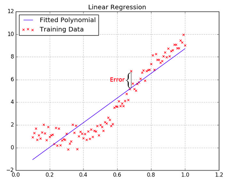
Linear regression is a method used to find a relationship between a dependent variable and a set of independent variables. In its simplest form it consist of fitting a function $ \boldsymbol{y} = w.\boldsymbol{x}+b $ to observed data, where $\boldsymbol{y}$ is the dependent variable, $\boldsymbol{x}$ the independent, $w$ the weight matrix and $b$ the bias.
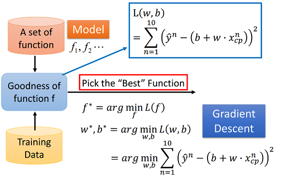
The goal is to find a best function by utilizing gradient descent to minimize the loss function
Given a function defined by a set of parameters, gradient descent starts with an initial set of parameter values and iteratively moves toward a set of parameter values that minimize the function. This iterative minimization is achieved using calculus, taking steps in the negative direction of the function gradient.
import numpy as np
import matplotlib
import matplotlib.pyplot as plt
# y_data = b + w * x_data
x_data = [338., 333., 328., 207., 226., 25., 179., 60., 208., 606.]
y_data = [640., 633., 619., 393., 428., 27., 193., 66., 226., 1591.]
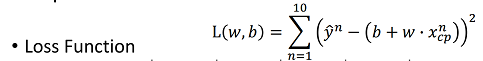
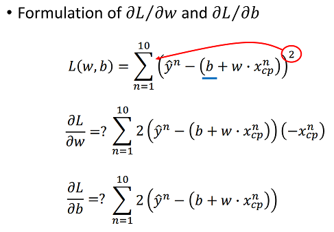
Loss Function: the sum of square of the difference between predicted output and actual output. It is a way to map the performance of our model into a real number. It measures how well the model is performing its task, be it a linear regression model fitting the data to a line, a neural network correctly classifying an image of a character, etc. The loss function is particularly important in learning since it is what guides the update of the parameters so that the model can perform better.
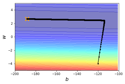
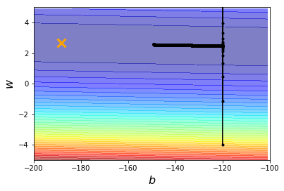
x = np.arange(-200, -100, 1) #bias
y = np.arange(-5,5,0.1) #weight
Z = np.zeros((len(x), len(y)))
X, Y = np.meshgrid(x, y)

for i in range(len(x)):
    for j in range(len(y)):
        b = x[i]
        w = y[j]
        Z[j][i] = 0
        for n in range(len(x_data)):
            Z[j][i] = Z[j][i] + (y_data[n] - b - w * x_data[n])**2     #loss function
        Z[j][i] = Z[j][i]/len(x_data)
# y_data = b + w * x_data
b = -120 # intial b
w = -4 # initial w
lr = 0.000001 # learning rate
iteration  = 100000

# store inital value for plotting
b_history = [b]
w_history = [w]

#iteration
for i in range(iteration):

    b_grad = 0.0
    w_grad = 0.0
    for n in range(len(x_data)):
        w_grad = w_grad - 2.0 * (y_data[n] - b - w * x_data[n]) * x_data[n]    #check the above formula
        b_grad = b_grad - 2.0 * (y_data[n] - b - w * x_data[n]) * 1.0          #check the above formula

    # udpate parameters
    b = b - lr * b_grad
    w = w - lr * w_grad

    # store parameters for plotting
    b_history.append(b)
    w_history.append(w)


# plot the figures
plt.contourf(x,y,Z, 50, alpha = 0.5, cmap=plt.get_cmap('jet'))
plt.plot([-188.4],[2.67], 'x', ms=12, markeredgewidth = 3, color = 'orange')
plt.plot(b_history, w_history, 'o-', ms =3, lw =1.5, color ='black')
plt.xlim(-200, -100)
plt.ylim(-5,5)
plt.xlabel(r'$b$', fontsize = 16)
plt.ylabel(r'$w$', fontsize = 16)
plt.show()
define a new learning rate = 1, define a new learning rate, and update parameter
# y_data = b + w * x_data
b = -120 # intial b
w = -4 # initial w
lr = 1 # learning rate   <-----
iteration  = 100000

# store inital value for plotting
b_history = [b]
w_history = [w]

# new defined  <---
lr_b = 0
lr_w = 0

#iteration
for i in range(iteration):

    b_grad = 0.0
    w_grad = 0.0
    for n in range(len(x_data)):
        b_grad = b_grad - 2.0 * (y_data[n] - b - w * x_data[n]) * 1.0
        w_grad = w_grad - 2.0 * (y_data[n] - b - w * x_data[n]) * x_data[n]

    # define a new learning rate   <----
    lr_b = lr_b + b_grad ** 2
    lr_w = lr_w + w_grad ** 2

    # update parameters   <----
    b = b - lr/np.sqrt(lr_b) * b_grad
    w = w - lr/np.sqrt(lr_w) * w_grad

    # store parameters for plotting
    b_history.append(b)
    w_history.append(w)


# plot the figures
plt.contourf(x,y,Z, 50, alpha = 0.5, cmap=plt.get_cmap('jet'))
plt.plot([-188.4],[2.67], 'x', ms=12, markeredgewidth = 3, color = 'orange')
plt.plot(b_history, w_history, 'o-', ms =3, lw =1.5, color ='black')
plt.xlim(-200, -100)
plt.ylim(-5,5)
plt.xlabel(r'$b$', fontsize = 16)
plt.ylabel(r'$w$', fontsize = 16)
plt.show()