01 Basics
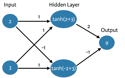
Forward propagation

import numpy as np
input_data = np.array([2,3])
weights = {'node_0': np.array([1,1]),
           'node_1': np.array([-1,1]),
           'output': np.array([2,-1])}
node_0_value = (input_data * weights['node_0']).sum()
node_1_value = (input_data * weights['node_1']).sum()

hidden_layer_values = np.array([node_0_value, node_1_value])
print(hidden_layer_values)

output = (hidden_layer_values * weights['output']).sum()
print(output)
[5 1]
9
Activation functions
An “activation function” is a function applied at each node. It converts the node’s input into some output.
import numpy as np
input_data = np.array([2,3])
weights = {'node_0': np.array([1,1]),
           'node_1': np.array([-1,1]),
           'output': np.array([2,-1])}

node_0_input = (input_data * weights['node_0']).sum()
node_0_output = np.tanh(node_0_input)

node_1_input = (input_data * weights['node_1']).sum()
node_1_output = np.tanh(node_1_input)

hidden_layer_values = np.array([node_0_output, node_1_output])
print(hidden_layer_values)

output = (hidden_layer_values * weights['output']).sum()
print(output)
[ 0.9999092   0.76159416]
1.23822425257
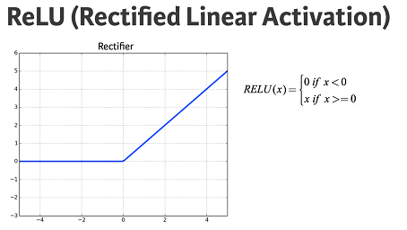
The rectified linear activation function (called ReLU) has been shown to lead to very high-performance networks. This function takes a single number as an input, returning 0 if the input is negative, and the input if the input is positive.
def relu(input):
    '''Define your relu activation function here'''
    # Calculate the value for the output of the relu function: output
    output = max(input, 0)

    # Return the value just calculated
    return(output)
import numpy as np
input_data = np.array([-1,2])
weights = {'node_0': np.array([3,3]),
           'node_1': np.array([1,5]),
           'output': np.array([2,-1])}

node_0_input = (input_data * weights['node_0']).sum()
node_0_output = relu(node_0_input)

node_1_input = (input_data * weights['node_1']).sum()
node_1_output = relu(node_1_input)

hidden_layer_values = np.array([node_0_output, node_1_output])
print(hidden_layer_values)

output = (hidden_layer_values * weights['output']).sum()
print(output)
[3 9]
-3
Applying the network to many observations/rows of data
Define a function called predict_with_network() which will generate predictions for multiple data observations
input_data = np.array([[3,5],[2,-1],[0,0],[8,4]])
input_data

# Define predict_with_network(), and return a prediction from the network as the output.
def predict_with_network(input_data_row, weights):

    # Calculate node 0 value. To calculate the input value of a node, multiply the relevant
    # arrays together and compute their sum
    node_0_input = (input_data_row * weights['node_0']).sum()
    node_0_output = relu(node_0_input)

    # Calculate node 1 value
    node_1_input = (input_data_row * weights['node_1']).sum()
    node_1_output = relu(node_1_input)

    # Put node values into array: hidden_layer_outputs
    hidden_layer_outputs = np.array([node_0_output, node_1_output])

    # Calculate model output
    input_to_final_layer = (hidden_layer_outputs * weights['output']).sum()
    model_output = relu(input_to_final_layer)

    # Return model output
    return(model_output)


# Create empty list to store prediction results
results = []
for input_data_row in input_data:
    # Append prediction to results
    results.append(predict_with_network(input_data_row, weights))

# Print results
print(results)
[20, 6, 0, 44]
Multi-layer neural networks
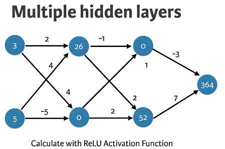
input_data = np.array([3,5])

weights = {'node_0_0': np.array([2,4]),
           'node_0_1': np.array([4,-5]),
           'node_1_0': np.array([-1,1]),
           'node_1_1': np.array([2,2]),
           'output': np.array([-3,7])}


def predict_with_network2(input_data):
    # Calculate node 0 in the first hidden layer
    node_0_0_input = (input_data * weights['node_0_0']).sum()
    node_0_0_output = relu(node_0_0_input)

    # Calculate node 1 in the first hidden layer
    node_0_1_input = (input_data * weights['node_0_1']).sum()
    node_0_1_output = relu(node_0_1_input)

    # Put node values into array: hidden_0_outputs
    hidden_0_outputs = np.array([node_0_0_output, node_0_1_output])
    print(hidden_0_outputs)

    # Calculate node 0 in the second hidden layer
    node_1_0_input = (hidden_0_outputs * weights['node_1_0']).sum()
    node_1_0_output = relu(node_1_0_input)

    # Calculate node 1 in the second hidden layer
    node_1_1_input = (hidden_0_outputs * weights['node_1_1']).sum()
    node_1_1_output = relu(node_1_1_input)

    # Put node values into array: hidden_1_outputs
    hidden_1_outputs = np.array([node_1_0_output, node_1_1_output])
    print(hidden_1_outputs)

    # Calculate model output: model_output
    model_output = (hidden_1_outputs * weights['output']).sum()


    # Return model_output
    return(model_output)

output = predict_with_network2(input_data)
print(output)
[26  0]
[ 0 52]
364
02 Opitimization
How weight changes affect accuracy
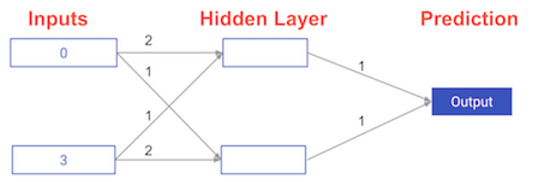
# The data point you will make a prediction for
input_data = np.array([0, 3])

# Sample weights
weights_0 = {'node_0': [2, 1],
             'node_1': [1, 2],
             'output': [1, 1]
            }

# The actual target value, used to calculate the error
target_actual = 3

# Make prediction using original weights, this was defined previously
predict_with_network(input_data, weights_0)
model_output_0 = predict_with_network(input_data, weights_0)

# Calculate error: error_0
error_0 = model_output_0 - target_actual

# Create weights that cause the network to make perfect prediction (3): weights_1
weights_1 = {'node_0': [2, 1],
             'node_1': [1, 0],   #change only one weight to ensure 0 error
             'output': [1, 1]
            }


# Make prediction using new weights: model_output_1
model_output_1 = predict_with_network(input_data, weights_1)


# Calculate error: error_1
error_1 = model_output_1 - target_actual

# Print error_0 and error_1
print(error_0)
print(error_1)
6
0
Scaling up to multiple data points
measure model accuracy on many points
import numpy as np
from sklearn.metrics import mean_squared_error
# The data point you will make a prediction for
input_data = np.array(([0, 3],[1,2],[-1,-2],[4,0]))

# Sample weights
weights_0 = {'node_0': [2, 1],
             'node_1': [1, 2],
             'output': [1, 1]
            }

weights_1 = {'node_0': [2, 1],
             'node_1': [1., 1.5],
             'output': [1., 1.5]
            }

#target_actuals = np.array([1,3,5,7])
target_actuals = ([1,3,5,7])
target_actuals
[1, 3, 5, 7]
# Create model_output_0
model_output_0 = []
# Create model_output_0
model_output_1 = []

# Loop over input_data
for row in input_data:
    # Append prediction to model_output_0
    model_output_0.append(predict_with_network(row, weights_0))

    # Append prediction to model_output_1
    model_output_1.append(predict_with_network(row, weights_1))

# Calculate the mean squared error for model_output_0: mse_0
mse_0 = mean_squared_error(target_actuals, model_output_0)

# Calculate the mean squared error for model_output_1: mse_1
mse_1 = mean_squared_error(target_actuals, model_output_1)

# Print mse_0 and mse_1
print("Mean squared error with weights_0: %f" %mse_0)
print("Mean squared error with weights_1: %f" %mse_1)
Mean squared error with weights_0: 37.500000
Mean squared error with weights_1: 49.890625
Gradient descent
When plotting the mean-squared error loss function against predictions, the slope is \begin{equation} 2 \times X \times (Y-Xb) \end{equation} \begin{equation} 2 \times InputData \times Error. \end{equation}
Note that X and B may have multiple numbers (X is a vector for each data point, and B is a vector). In this case, the output will also be a vector, which is exactly what you want.
Gradient descent_01 Calculating slopes
import numpy as np
weights = np.array([0,2,1])
input_data = np.array([1,2,3])
target = 0


# Calculate the predictions: preds
preds = (weights * input_data).sum()

# Calculate the error: error (Notice that this error corresponds to y-xb in the gradient expression.)
error =  preds - target

# Calculate the slope of the loss function with respect to the prediction.
slope = 2 * input_data * error

# Print the slope
print(slope)
[14 28 42]
Gradient descent_02 Improving model weights
# Set the learning rate: learning_rate
learning_rate = 0.01

# Update the weights: weights_updated
weights_updated = weights - learning_rate * slope

# Get updated predictions: preds_updated
preds_updated = (weights_updated * input_data).sum()

# Calculate updated error: error_updated
error_updated = preds_updated - target

# Print the original error
print(error)

# Print the updated error
print(error_updated)
7
5.04
Gradient descent_03 Making multiple updates to weights