1. SVM支持向量机:
The princile of SVM is to find out hyper plan between two classes of datasets.
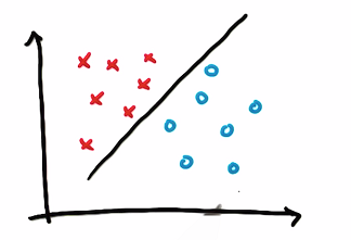
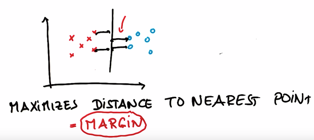
What this line does that the other ones don’t do? It maximizes the distance to the nearest point, and it does this relative to both classes.
It’s a line that maximizes the distance to the nearest points in either class, that distance is often called margin. The margin is the distance between the line and the nearest point of either of the two classes.
Two key points:
- SVM always consider whether the classification is correct or not, rather than maximizing the distance between datasets.
- SVM maximizes the robustness of the classification.
- SVM looks for the decision surface that maxmizes the distance of two datasets, meanwhile tolerates specific outliner by parameter tuning.
2. SVM in SKLEARN
http://scikit-learn.org/stable/modules/svm.html
from sklearn import svm
X = [[0, 0], [1, 1]]  # training feature
y = [0, 1]            # training label
clf = svm.SVC()       # create classifier
clf.fit(X, y)         # training
SVC(C=1.0, cache_size=200, class_weight=None, coef0=0.0,
  decision_function_shape=None, degree=3, gamma='auto', kernel='rbf',
  max_iter=-1, probability=False, random_state=None, shrinking=True,
  tol=0.001, verbose=False)
clf.predict([[2., 2.]]) #the model can then be used to predict new values
array([1])
Coding up with SVM
import sys
from class_vis import prettyPicture
from prep_terrain_data import makeTerrainData

import matplotlib.pyplot as plt
import copy
import numpy as np
import pylab as pl


features_train, labels_train, features_test, labels_test = makeTerrainData()


########################## SVM #################################
### we handle the import statement and SVC creation for you here
from sklearn.svm import SVC
clf = SVC(kernel="linear")


#### now your job is to fit the classifier
#### using the training features/labels, and to
#### make a set of predictions on the test data

clf.fit(features_train, labels_train)

#### store your predictions in a list named pred
pred = clf.predict(features_test)    #only input features_test because the label is what we are trying to predict

from sklearn.metrics import accuracy_score
acc = accuracy_score(pred, labels_test)

def submitAccuracy():
    return acc
acc
0.92000000000000004
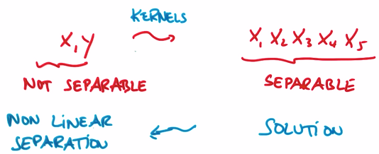
3. Non-Linear SVM
Z represents the distance from origin. Mapping dataset to the coordinate which has Z, you will find the blue circle has bigger Z value, red circle has smaller Z value: i.e. linearly separable in the new coordinate.
Therefore, SVM can learn non-linear decision from round by adding Z
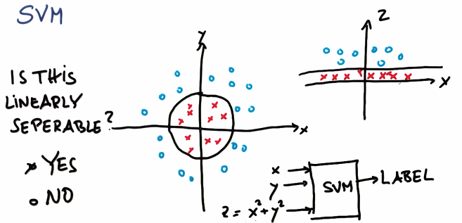
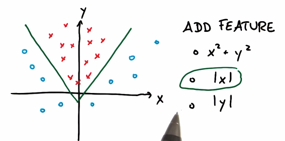
kernal trick
To avoid developing a bundle of new features, we use kernal trick: accept input or features with lower dimension, mapping them into high dimensions.
应用核函数将输入空间从xy变换到更大的输入空间后,再使用SVM对数据点分类,得到解后返回原始空间,得到一个非线性分割。
4. SVM in SKLEARN
http://scikit-learn.org/stable/modules/generated/sklearn.svm.SVC.html
Parameter:
- Kernal
- Gamma, 单个训练样本,对结果作用范围的远近(define how far the influence of a single training example reaches)
- 较小值意味着每个点都可能对最终结果产生作用
- 较大值意味着训练样本对距离较近的决策边界有影响
- C, 在光滑的决策边界,以及尽可能正确分类所有训练点两者之间进行平衡. C值越大,就得到更复杂的决策边界值.
import sys
from class_vis import prettyPicture
from prep_terrain_data import makeTerrainData

import matplotlib.pyplot as plt
import copy
import numpy as np
import pylab as pl


features_train, labels_train, features_test, labels_test = makeTerrainData()


########################## SVM #################################
### we handle the import statement and SVC creation for you here
from sklearn.svm import SVC
clf = SVC(kernel="rbf", C=1000)


#### now your job is to fit the classifier
#### using the training features/labels, and to
#### make a set of predictions on the test data

clf.fit(features_train, labels_train)

#### store your predictions in a list named pred
pred = clf.predict(features_test)    #only input features_test because the label is what we are trying to predict

from sklearn.metrics import accuracy_score
acc = accuracy_score(pred, labels_test)

def submitAccuracy():
    return acc
acc
0.92400000000000004
5. Pros and Cons
Pros:
- suitable for complex dataset with clearly delimited boundaries
Cons
- Not suitable massive data: the training time is proportional to the third power of data volume
- Not suitable to the dataset which has too much noises (naive bayes is more suitable)
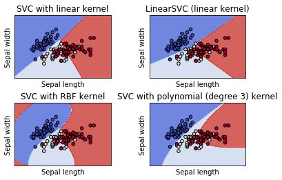
6. Plot different SVM classifiers in the iris dataset
Comparison of different linear SVM classifiers on a 2D projection of the iris dataset. We only consider the first 2 features of this dataset:
- Sepal length
- Sepal width
This example shows how to plot the decision surface for four SVM classifiers with different kernels.
print(__doc__)

import numpy as np
import matplotlib.pyplot as plt
from sklearn import svm, datasets


def make_meshgrid(x, y, h=.02):
    """Create a mesh of points to plot in

    Parameters
    ----------
    x: data to base x-axis meshgrid on
    y: data to base y-axis meshgrid on
    h: stepsize for meshgrid, optional

    Returns
    -------
    xx, yy : ndarray
    """
    x_min, x_max = x.min() - 1, x.max() + 1
    y_min, y_max = y.min() - 1, y.max() + 1
    xx, yy = np.meshgrid(np.arange(x_min, x_max, h),
                         np.arange(y_min, y_max, h))
    return xx, yy


def plot_contours(ax, clf, xx, yy, **params):
    """Plot the decision boundaries for a classifier.

    Parameters
    ----------
    ax: matplotlib axes object
    clf: a classifier
    xx: meshgrid ndarray
    yy: meshgrid ndarray
    params: dictionary of params to pass to contourf, optional
    """
    Z = clf.predict(np.c_[xx.ravel(), yy.ravel()])
    Z = Z.reshape(xx.shape)
    out = ax.contourf(xx, yy, Z, **params)
    return out


# import some data to play with
iris = datasets.load_iris()
# Take the first two features. We could avoid this by using a two-dim dataset
X = iris.data[:, :2]
y = iris.target

# we create an instance of SVM and fit out data. We do not scale our
# data since we want to plot the support vectors
C = 1.0  # SVM regularization parameter
models = (svm.SVC(kernel='linear', C=C),
          svm.LinearSVC(C=C),
          svm.SVC(kernel='rbf', gamma=0.7, C=C),
          svm.SVC(kernel='poly', degree=3, C=C))
models = (clf.fit(X, y) for clf in models)

# title for the plots
titles = ('SVC with linear kernel',
          'LinearSVC (linear kernel)',
          'SVC with RBF kernel',
          'SVC with polynomial (degree 3) kernel')

# Set-up 2x2 grid for plotting.
fig, sub = plt.subplots(2, 2)
plt.subplots_adjust(wspace=0.4, hspace=0.4)

X0, X1 = X[:, 0], X[:, 1]
xx, yy = make_meshgrid(X0, X1)

for clf, title, ax in zip(models, titles, sub.flatten()):
    plot_contours(ax, clf, xx, yy,
                  cmap=plt.cm.coolwarm, alpha=0.8)
    ax.scatter(X0, X1, c=y, cmap=plt.cm.coolwarm, s=20, edgecolors='k')
    ax.set_xlim(xx.min(), xx.max())
    ax.set_ylim(yy.min(), yy.max())
    ax.set_xlabel('Sepal length')
    ax.set_ylabel('Sepal width')
    ax.set_xticks(())
    ax.set_yticks(())
    ax.set_title(title)

plt.show()
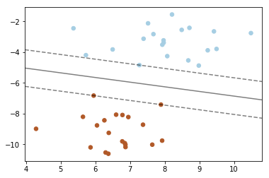
7. SVM: Maximum margin separating hyperplane
Plot the maximum margin separating hyperplane within a two-class separable dataset using a Support Vector Machine classifier with linear kernel.
print(__doc__)

import numpy as np
import matplotlib.pyplot as plt
from sklearn import svm
from sklearn.datasets import make_blobs


# we create 40 separable points
X, y = make_blobs(n_samples=40, centers=2, random_state=6)

# fit the model, don't regularize for illustration purposes
clf = svm.SVC(kernel='linear', C=1000)
clf.fit(X, y)

plt.scatter(X[:, 0], X[:, 1], c=y, s=30, cmap=plt.cm.Paired)

# plot the decision function
ax = plt.gca()
xlim = ax.get_xlim()
ylim = ax.get_ylim()

# create grid to evaluate model
xx = np.linspace(xlim[0], xlim[1], 30)
yy = np.linspace(ylim[0], ylim[1], 30)
YY, XX = np.meshgrid(yy, xx)
xy = np.vstack([XX.ravel(), YY.ravel()]).T
Z = clf.decision_function(xy).reshape(XX.shape)

# plot decision boundary and margins
ax.contour(XX, YY, Z, colors='k', levels=[-1, 0, 1], alpha=0.5,
           linestyles=['--', '-', '--'])
# plot support vectors
ax.scatter(clf.support_vectors_[:, 0], clf.support_vectors_[:, 1], s=100,
           linewidth=1, facecolors='none')
plt.show()