Clustering via 𝑘 -means

Clustering via 𝑘 means

In many applications, the data have no labels but we wish to discover possible labels (or other hidden patterns or structures). This problem is one of unsupervised learning. How can we approach such problems?

Clustering is one class of unsupervised learning methods.

import requests
import os
import hashlib
import io

The 𝑘 -means clustering criterion

One way to measure the quality of a set of clusters: For each cluster 𝐶 , consider its center 𝜇 and measure the distance ‖𝑥−𝜇‖ of each observation 𝑥∈𝐶 to the center. Add these up for all points in the cluster; call this sum is the within-cluster sum-of-squares (WCSS). Then, set as our goal to choose clusters that minimize the total WCSS over all clusters.

More formally, given a clustering $C = {C_0, C_1, \ldots, C_{k-1}}$, let

$\mathrm{WCSS}(C) \equiv \sum_{i=0}^{k-1} \sum_{x\in C_i} \|x - \mu_i\|^2,$

where $\mu_i$ is the center of $C_i$. This center may be computed simply as the mean of all points in $C_i$, i.e.,

$\mu_i \equiv \dfrac{1}{|C_i|} \sum_{x \in C_i} x.$

Then, our objective is to find the “best” clustering, $C_*$, which is the one that has a minimum WCSS.

$C_* = \arg\min_C \mathrm{WCSS}(C).$

The standard $k$-means algorithm (Lloyd’s algorithm)

Finding the global optimum is NP-hard, which is computer science mumbo jumbo for “we don’t know whether there is an algorithm to calculate the exact answer in fewer steps than exponential in the size of the input.” Nevertheless, there is an iterative method, Lloyd’s algorithm, that can quickly converge to a local (as opposed to global) minimum. The procedure alternates between two operations: assignment and update.

Step 1: Assignment. Given a fixed set of $k$ centers, assign each point to the nearest center:

$C_i = \{\hat{x}: \| \hat{x} - \mu_i \| \le \| \hat{x} - \mu_j \|, 1 \le j \le k \}.$

Step 2: Update. Recompute the $k$ centers (“centroids”) by averaging all the data points belonging to each cluster, i.e., taking their mean:

$\mu_i = \dfrac{1}{|C_i|} \sum_{\hat{x} \in C_i} \hat{x}$

Illustration of $k$-means

> Figure adapted from: http://stanford.edu/~cpiech/cs221/img/kmeansViz.png

import numpy as np
import pandas as pd
import seaborn as sns
import matplotlib.pyplot as plt

%matplotlib inline

import matplotlib as mpl
mpl.rc("savefig", dpi=100) # Adjust for higher-resolution figures

df = pd.read_csv('{}logreg_points_train.csv'.format(DATA_PATH))
df.head()

	x_1	x_2	label
0	-0.234443	-1.075960	1
1	0.730359	-0.918093	0
2	1.432270	-0.439449	0
3	0.026733	1.050300	0
4	1.879650	0.207743	0

def make_scatter_plot(df, x="x_1", y="x_2", hue="label",
                      palette={0: "red", 1: "olive"},
                      size=5,
                      centers=None):
    sns.lmplot(x=x, y=y, hue=hue, data=df, palette=palette,
               fit_reg=False)
    if centers is not None:
        plt.scatter(centers[:,0], centers[:,1],
                    marker=u'*', s=500,
                    c=[palette[0], palette[1]])
    
def mark_matches(a, b, exact=False):
    """
    Given two Numpy arrays of {0, 1} labels, returns a new boolean
    array indicating at which locations the input arrays have the
    same label (i.e., the corresponding entry is True).
    
    This function can consider "inexact" matches. That is, if `exact`
    is False, then the function will assume the {0, 1} labels may be
    regarded as the same up to a swapping of the labels. This feature
    allows
    
      a == [0, 0, 1, 1, 0, 1, 1]
      b == [1, 1, 0, 0, 1, 0, 0]
      
    to be regarded as equal. (That is, use `exact=False` when you
    only care about "relative" labeling.)
    """
    assert a.shape == b.shape
    a_int = a.astype(dtype=int)
    b_int = b.astype(dtype=int)
    all_axes = tuple(range(len(a.shape)))
    assert ((a_int == 0) | (a_int == 1)).all()
    assert ((b_int == 0) | (b_int == 1)).all()
    
    exact_matches = (a_int == b_int)
    if exact:
        return exact_matches

    assert exact == False
    num_exact_matches = np.sum(exact_matches)
    if (2*num_exact_matches) >= np.prod (a.shape):
        return exact_matches
    return exact_matches == False # Invert
    
def count_matches(a, b, exact=False):
    """
    Given two sets of {0, 1} labels, returns the number of mismatches.
    
    This function can consider "inexact" matches. That is, if `exact`
    is False, then the function will assume the {0, 1} labels may be
    regarded as similar up to a swapping of the labels. This feature
    allows
    
      a == [0, 0, 1, 1, 0, 1, 1]
      b == [1, 1, 0, 0, 1, 0, 0]
      
    to be regarded as equal. (That is, use `exact=False` when you
    only care about "relative" labeling.)
    """
    matches = mark_matches(a, b, exact=exact)
    return np.sum(matches)

make_scatter_plot(df)

png

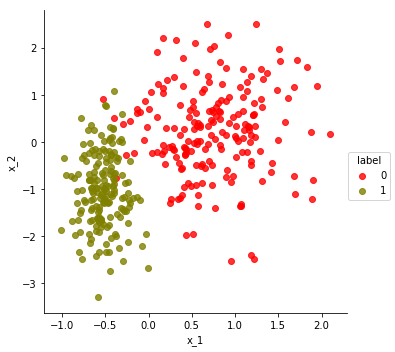
Let’s extract the data points as a data matrix, points, and the labels as a vector, labels. Note that the k-means algorithm you will implement should not reference labels – that’s the solution we will try to predict given only the point coordinates (points) and target number of clusters (k).

points = df[['x_1', 'x_2']].values
labels = df['label'].values
n, d = points.shape
k = 2

Initializing the 𝑘 centers

Step 01: randomly choose 𝑘 observations from the data.

The below function randomly selects $k$ of the given observations to serve as centers. It should return a Numpy array of size k-by-d, where d is the number of columns of X.

def init_centers(X, k):

    from numpy.random import choice
    sample = choice(len(X), size = k, replace = False)
    return X[sample, : ]

step 02: Computing the distances

The below function computes a distance matrix, $S = (s_{ij})$ such that $s_{ij} = d_{ij}^2$ is the squared distance from point $\hat{x}_i$ to center $\mu_j$. It should return a Numpy matrix S[:m, :k].

def compute_d2(X, centers):
    
    return np.linalg.norm(X[:, np.newaxis, :] - centers, ord=2, axis=2) ** 2

step 03: uses the (squared) distance matrix to assign a “cluster label” to each point.

That is, consider the $m \times k$ squared distance matrix $S$. For each point $i$, if $s_{i,j}$ is the minimum squared distance for point $i$, then the index $j$ is $i$’s cluster label. In other words, your function should return a (column) vector $y$ of length $m$ such that

$y_i = \underset{j \in \{0, \ldots, k-1\}}{\operatorname{argmin}} s_{ij}.$

def assign_cluster_labels(S):
    
    return np.argmin(S, axis=1)
# Cluster labels:     0    1
S_test1 = np.array([[0.3, 0.2],  # --> cluster 1
                    [0.1, 0.5],  # --> cluster 0
                    [0.4, 0.2]]) # --> cluster 1
y_test1 = assign_cluster_labels(S_test1)
print("You found:", y_test1)

assert (y_test1 == np.array([1, 0, 1])).all()

You found: [1 0 1]

step 04: Given a clustering (i.e., a set of points and assignment of labels), compute the center of each cluster.

def update_centers(X, y):
    # X[:m, :d] == m points, each of dimension d
    # y[:m] == cluster labels
    m, d = X.shape
    k = max(y) + 1
    assert m == len(y)
    assert (min(y) >= 0)
    
    centers = np.empty((k, d))
    for j in range(k):
    
        centers[j, :d] = np.mean(X[y == j, :], axis=0)
    return centers

step 05: Given the squared distances, return the within-cluster sum of squares.

In particular, the function should have the signature,

    def WCSS(S):
        ...

where S is an array of distances as might be computed from Exercise 2.

For example, suppose S is defined as follows:

    S = np.array([[0.3, 0.2],
                  [0.1, 0.5],
                  [0.4, 0.2]])

Then WCSS(S) == 0.2 + 0.1 + 0.2 == 0.5.

def WCSS(S):
    return np.sum(np.amin(S, axis = 1))
# Quick test:
print("S ==\n", S_test1)
WCSS_test1 = WCSS(S_test1)
print("\nWCSS(S) ==", WCSS(S_test1))

S ==
 [[0.3 0.2]
 [0.1 0.5]
 [0.4 0.2]]

WCSS(S) == 0.5

The below function checks whether the centers have “moved,” given two instances of the center values. It accounts for the fact that the order of centers may have changed.

def has_converged(old_centers, centers):
    return set([tuple(x) for x in old_centers]) == set([tuple(x) for x in centers])

step 06: Put all of the preceding building blocks together to implement Lloyd’s 𝑘 -means algorithm.

def kmeans(X, k,
           starting_centers=None,
           max_steps=np.inf):
    if starting_centers is None:
        centers = init_centers(X, k)
    else:
        centers = starting_centers
        
    converged = False
    labels = np.zeros(len(X))
    i = 1
    while (not converged) and (i <= max_steps):
        old_centers = centers
        
        S = compute_d2(X, centers)
        labels = assign_cluster_labels(S)
        centers = update_centers(X, labels)
        converged = has_converged(old_centers, centers)
        
        print ("iteration", i, "WCSS = ", WCSS (S))
        i += 1
    return labels

clustering = kmeans(points, k, starting_centers=points[[0, 187], :])

iteration 1 WCSS =  549.9175535488309
iteration 2 WCSS =  339.80066330255096
iteration 3 WCSS =  300.330112922328
iteration 4 WCSS =  289.80700777322045
iteration 5 WCSS =  286.0745591062787
iteration 6 WCSS =  284.1907705579879
iteration 7 WCSS =  283.22732249939105
iteration 8 WCSS =  282.456491302569
iteration 9 WCSS =  281.84838225337074
iteration 10 WCSS =  281.57242082723724
iteration 11 WCSS =  281.5315627987326

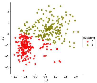
Let us visualize the result

df['clustering'] = clustering
centers = update_centers(points, clustering)
make_scatter_plot(df, hue='clustering', centers=centers)

n_matches = count_matches(df['label'], df['clustering'])
print(n_matches,
      "matches out of",
      len(df), "possible",
      "(~ {:.1f}%)".format(100.0 * n_matches / len(df)))

assert n_matches >= 320

329 matches out of 375 possible (~ 87.7%)

png

Clustering via 𝑘 -means