Basic concepts of Bayesian methods

What is Naive Bayes?

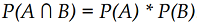
Naive Bayes assumes class-conditional independence, which means that events are independent so long as they are conditioned on the same class value.

The probability of both happening is: png

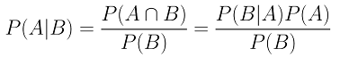
Conditional probability png

Case example:

png

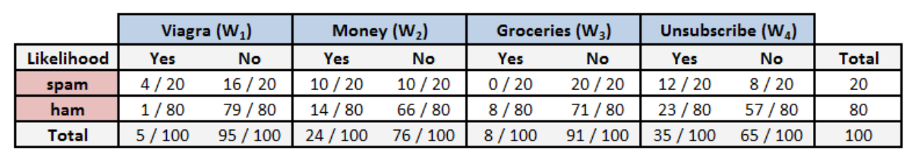
The probability that a message is spam, given that Viagra = Yes, Money = No, Groceries = No, and Unsubscribe = Yes:

probability that the message is spam: =(4/20)*(10/20)*(20/20)*(12/20)*(20/100)=0.012
probability that the message is ham: =(1/80)*(66/80)*(71/80)*(23/80)*(80/100)=0.002

Because 0.012 / 0.002 = 6, we can say that this message is six times more likely to be spam than ham. However, to convert these numbers to probabilities, we need one last step. The probability of spam is equal to the likelihood that the message is spam divided by the likelihood that the message is either spam or ham:

=0.012/(0.012 + 0.002)=0.857

Similarly, the probability of ham is equal to the likelihood that the message is ham divided by the likelihood that the message is either spam or ham:

=0.002/(0.012 + 0.002)=0.143

In summary, given the pattern of words in the message, we expect that the message is spam with 85.7 percent probability, and ham with 14.3 percent probability. Because these are mutually exclusive and exhaustive events, the probabilities sum up to one.

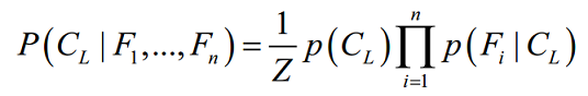
The naive Bayes classification algorithm

Essentially, the probability of level L for class C, given the evidence provided by features F1 through Fn, is equal to the product of the probabilities of each piece of evidence conditioned on the class level, the prior probability of the class level, and a scaling factor 1 / Z, which converts the result to a probability:

png

The Laplace estimator

Case example 2

Given all Viagra, Groceries, Money, and Unsubscribe = YES

the likelihood of spam as:

(4/20)*(10/20)*(0/20)*(12/20)*(20/100)=0

And the likelihood of ham is:

(1/80)*(14/80)*(8/80)*(23/80)*(80/100)=0.00005

Therefore, the probability of spam is:

0/(0 + 0.0099)=0

And the probability of ham is:

0.00005/(0 + 0.0.00005)=1

These results suggest that the message is spam with 0 percent probability and ham with 100 percent probability. Does this prediction make sense? Probably not.

Because probabilities in naive Bayes are multiplied, this 0 percent value causes the posterior probability of spam to be zero, giving the word Groceries the ability to effectively nullify and overrule all of the other evidence

Solution

The Laplace estimator essentially adds a small number to each of the counts in the frequency

table, which ensures that each feature has a nonzero probability of occurring with each class. - Typically, the Laplace estimator is set to 1, which ensures that each class-feature combination is found in the data at least once.

The likelihood of spam is therefore:

(5/24)*(11/24)*(1/24)*(13/24)*(20/100)=0.0004

And the likelihood of ham is:

(2/84)*(15/84)*(9/84)*(24/84)*(80/100)=0.0001

In summary, this means that the probability of spam is 80 percent and the probability of ham is 20 percent; a more plausible result than the one obtained when Groceries alone determined the result.

Using numeric features with naive Bayes

Because naive Bayes uses frequency tables for learning the data, each feature must be categorical in order to create the combinations of class and feature values comprising the matrix. Since numeric features do not have categories of values, the preceding algorithm does not work directly with numeric data.

Solution

Discretize numeric features: This method is ideal when there are large amounts of training data, a common condition when working with naive Bayes. Explore the data for natural categories or cut points in the distribution of data.
One thing to keep in mind is that discretizing a numeric feature always results in a reduction of information, as the feature’s original granularity is reduced to a smaller number of categories. It is important to strike a balance, since too few bins can result in important trends being obscured, while too many bins can result in small counts in the naive Bayes frequency table.

Example

1. read raw material into sms_raw
2. convert "type" varaible from character to factor
3. create a corpus (sms_corpus) using sms_raw$text
4. clean the corpus to sms_corpus_clean by convert to lowercase, remove punctuation,remove 
number, remove filler word, stemming the word
5. create a data structure sms_dtm called a sparse matrix by tokenizing the cleaned corpus
6. split the data into a training dataset and test dataset
sms_dtm_train <- sms_dtm[1:4169, ]
sms_dtm_test <- sms_dtm[4170:5559, ]

sms_train_labels <- sms_raw[1:4169, ]$type
sms_test_labels <- sms_raw[4170:5559, ]$type

7. visualize the text data (wordcloud)
- visualize the cleaned corpus (sms_corpus_clean)
- visualize the sms_raw 

8. creating indicator features for frequent words from sms_dtm_train

9. filter DTM to include only the terms appearing in a specified vector.
sms_dtm_freq_train<- sms_dtm_train[ , sms_freq_words]
sms_dtm_freq_test <- sms_dtm_test[ , sms_freq_words]

10. change to a categorical variable that simply indicates yes or no depending on whether the 
word appears at all.
sms_train <- apply(sms_dtm_freq_train, MARGIN = 2, convert_counts)
sms_test <- apply(sms_dtm_freq_test, MARGIN = 2, convert_counts)

11. train a model
sms_classifier <- naiveBayes(sms_train, sms_train_labels)

12. Evaluate model performance
sms_test_pred <- predict(sms_classifier, sms_test)

13. Compare the predictions to the true values
CrossTable(sms_test_pred, sms_test_labels, prop.chisq = FALSE, prop.t = FALSE, dnn = c
('predicted', 'actual'))

14. Improve model performance with laplace = 1
sms_classifier2 <- naiveBayes(sms_train, sms_train_labels, laplace = 1)
sms_test_pred2 <- predict(sms_classifier2, sms_test)
CrossTable(sms_test_pred2, sms_test_labels, prop.chisq = FALSE, prop.t = FALSE, prop.r = FALSE,
dnn = c('predicted', 'actual'))

Example - filtering mobile phone spam with the naive Bayes algorithm

Step 1 - collecting data

data adapted from the SMS Spam Collection

Step 2 - exploring and preparing the data

We will transform our data into a representation known as bag-of-words, which ignores the order that words appear in and simply provides a variable indicating whether the word appears at all.

sms_raw <- read.csv("sms_spam.csv", stringsAsFactors = FALSE)
str(sms_raw)

## 'data.frame':    5559 obs. of  2 variables:
##  $ type: chr  "ham" "ham" "ham" "spam" ...
##  $ text: chr  "Hope you are having a good week. Just checking in" "K..give back my thanks." "Am also doing in cbe only. But have to pay." "complimentary 4 STAR Ibiza Holiday or Â£10,000 cash needs your URGENT collection. 09066364349 NOW from Landline not to lose out"| __truncated__ ...

The sms_raw data frame includes 5,559 total SMS messages with two features: type and text
The SMS type has been coded as either ham or spam, and the text variable stores the full raw SMS message text.

The type variable is currently a character vector. Since this is a categorical variable, it would be better to convert it to a factor,

sms_raw$type <- factor(sms_raw$type)
str(sms_raw$type)

##  Factor w/ 2 levels "ham","spam": 1 1 1 2 2 1 1 1 2 1 ...

table(sms_raw$type)

## 
##  ham spam 
## 4812  747

747 (or about 13 percent) of SMS messages were labeled spam, while the remainder were labeled ham:

Data preparation - processing text data for analysis

library(tm)

## Warning: package 'tm' was built under R version 3.3.3

## Loading required package: NLP

## Warning: package 'NLP' was built under R version 3.3.2

The first step in processing text data involves creating a corpus, which refers to a collection of text documents.

sms_corpus <- VCorpus(VectorSource(sms_raw$text))

Volatile corpus: volatile as it is stored in memory as opposed to being stored on disk (the PCorpus() function can be used to access a permanent corpus stored in a database).

# To learn more, examine the Data Import section in the tm package vignette
print(vignette("tm"))

5,559 SMS messages in the training data:

print(sms_corpus)

## <<VCorpus>>
## Metadata:  corpus specific: 0, document level (indexed): 0
## Content:  documents: 5559

Look at the contents of the corpus

inspect(sms_corpus[1:2])

## <<VCorpus>>
## Metadata:  corpus specific: 0, document level (indexed): 0
## Content:  documents: 2
## 
## [[1]]
## <<PlainTextDocument>>
## Metadata:  7
## Content:  chars: 49
## 
## [[2]]
## <<PlainTextDocument>>
## Metadata:  7
## Content:  chars: 23

# To view first document
as.character(sms_corpus[[1]])

## [1] "Hope you are having a good week. Just checking in"

# To view multiple documents
lapply(sms_corpus[2:4], as.character)

## $`2`
## [1] "K..give back my thanks."
## 
## $`3`
## [1] "Am also doing in cbe only. But have to pay."
## 
## $`4`
## [1] "complimentary 4 STAR Ibiza Holiday or Â£10,000 cash needs your URGENT collection. 09066364349 NOW from Landline not to lose out! Box434SK38WP150PPM18+"

Cleaning steps to remove punctuation and other characters that may clutter the result Convert all of the SMS messages to lowercase:

# corpus_clean <- tm_map(sms_corpus, (tolower))  # tm package 0.5.10
sms_corpus_clean <- tm_map(sms_corpus, content_transformer(tolower)) # tm package 0.6.2

# Test before/after
as.character(sms_corpus[[1]])

## [1] "Hope you are having a good week. Just checking in"

as.character(sms_corpus_clean[[1]])

## [1] "hope you are having a good week. just checking in"

Remove any numbers:

sms_corpus_clean <- tm_map(sms_corpus_clean, removeNumbers)

Remove filler words such as to, and, but, and or. These are known as stop words

sms_corpus_clean <- tm_map(sms_corpus_clean, removeWords, stopwords())

Remove punctuation:

sms_corpus_clean <- tm_map(sms_corpus_clean, removePunctuation)

Stemming: a process takes words like learned, learning, and learns, and strips the suffix in order to transform them into the base form, learn.

library(SnowballC)

## Warning: package 'SnowballC' was built under R version 3.3.2

ms_corpus_clean <- tm_map(sms_corpus_clean, stemDocument)

Remove additional whitespace, leaving only a single space between words.

sms_corpus_clean <- tm_map(sms_corpus_clean, stripWhitespace)

Look at the contents of the corpus AGAIN.

inspect(sms_corpus_clean[1:2])

## <<VCorpus>>
## Metadata:  corpus specific: 0, document level (indexed): 0
## Content:  documents: 2
## 
## [[1]]
## <<PlainTextDocument>>
## Metadata:  7
## Content:  chars: 29
## 
## [[2]]
## <<PlainTextDocument>>
## Metadata:  7
## Content:  chars: 17

lapply(sms_corpus[1:4], as.character)

## $`1`
## [1] "Hope you are having a good week. Just checking in"
## 
## $`2`
## [1] "K..give back my thanks."
## 
## $`3`
## [1] "Am also doing in cbe only. But have to pay."
## 
## $`4`
## [1] "complimentary 4 STAR Ibiza Holiday or Â£10,000 cash needs your URGENT collection. 09066364349 NOW from Landline not to lose out! Box434SK38WP150PPM18+"

Data preparation - splitting text documents into words

Tokenization: The DocumentTermMatrix() function will take a corpus and create a data structure called a sparse matrix, in which the rows of the matrix indicate documents (that is, SMS messages) and the columns indicate terms (that is, words). png

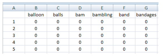
Create a sparse matrix given a tm corpus

sms_dtm <- DocumentTermMatrix(sms_corpus_clean)
sms_dtm

## <<DocumentTermMatrix (documents: 5559, terms: 7925)>>
## Non-/sparse entries: 42654/44012421
## Sparsity           : 100%
## Maximal term length: 40
## Weighting          : term frequency (tf)

This tokenizes the corpus and return the sparse matrix with the name sms_dtm.

Data preparation - creating training and test datasets

Split the data into a training dataset and test dataset

#sms_raw_train <- sms_raw[1:4169, ]
#sms_raw_test <- sms_raw[4170:5559, ]

sms_dtm_train <- sms_dtm[1:4169, ]
sms_dtm_test <- sms_dtm[4170:5559, ]

sms_train_labels <- sms_raw[1:4169, ]$type
sms_test_labels <- sms_raw[4170:5559, ]$type

prop.table(table(sms_train_labels))

## sms_train_labels
##       ham      spam 
## 0.8647158 0.1352842

prop.table(table(sms_test_labels))

## sms_test_labels
##       ham      spam 
## 0.8683453 0.1316547

Both the training data and test data contain about 13 percent spam. This suggests that the spam messages were divided evenly between the two datasets.

Visualizing text data - word clouds

library(wordcloud)

## Warning: package 'wordcloud' was built under R version 3.3.3

## Loading required package: RColorBrewer

## Warning: package 'RColorBrewer' was built under R version 3.3.2

#  A frequency of 50 is about 1 percent of the corpus, this means that a word must be found in at least 1 percent of the SMS messages to be included in the cloud 
wordcloud(sms_corpus_clean, min.freq=50, random.order = FALSE)

png

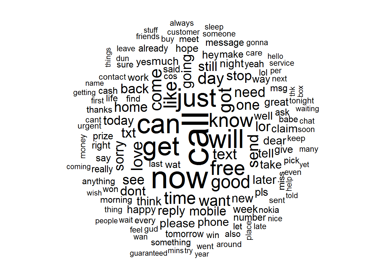
The cloud will be arranged in non-random order, with the higher-frequency words placed closer to the center
The min.freq parameter specifies the number of times a word must appear in the corpus before it will be displayed in the cloud. A general rule is to begin by setting min.freq to a number roughly 10 percent of the number of documents in the corpus

Visualization comparing the clouds for SMS spam and ham. Use the max.words parameter to look at the 40 most common words in each of the two sets. The scale parameter allows us to adjust the maximum and minimum font size for words in the cloud.

spam <- subset(sms_raw, type == "spam")
ham <- subset(sms_raw, type == "ham")

wordcloud(spam$text, max.words = 40, scale = c(3, 0.5))

png

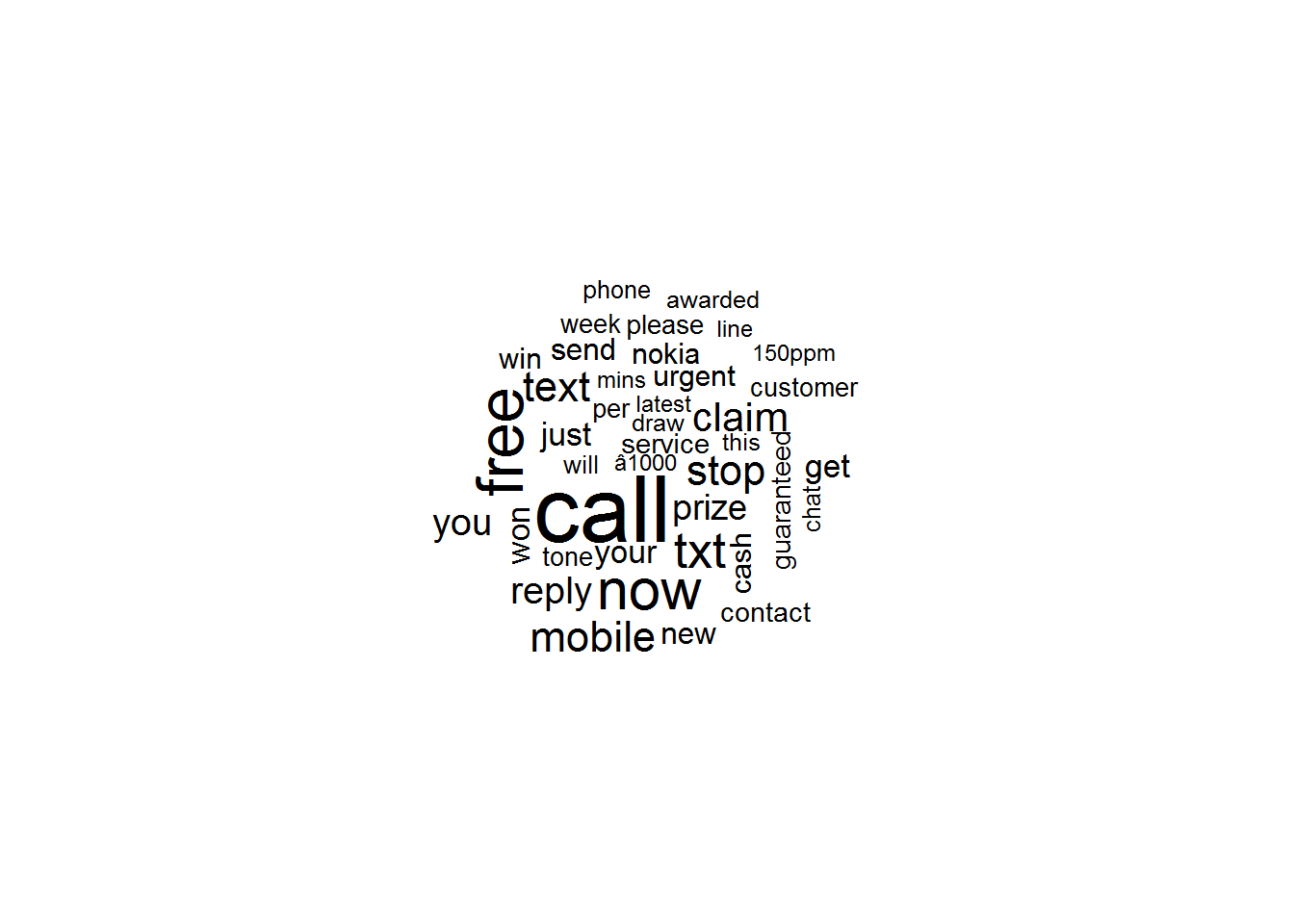
the spam cloud

wordcloud(ham$text, max.words = 40, scale = c(3, 0.5))

png

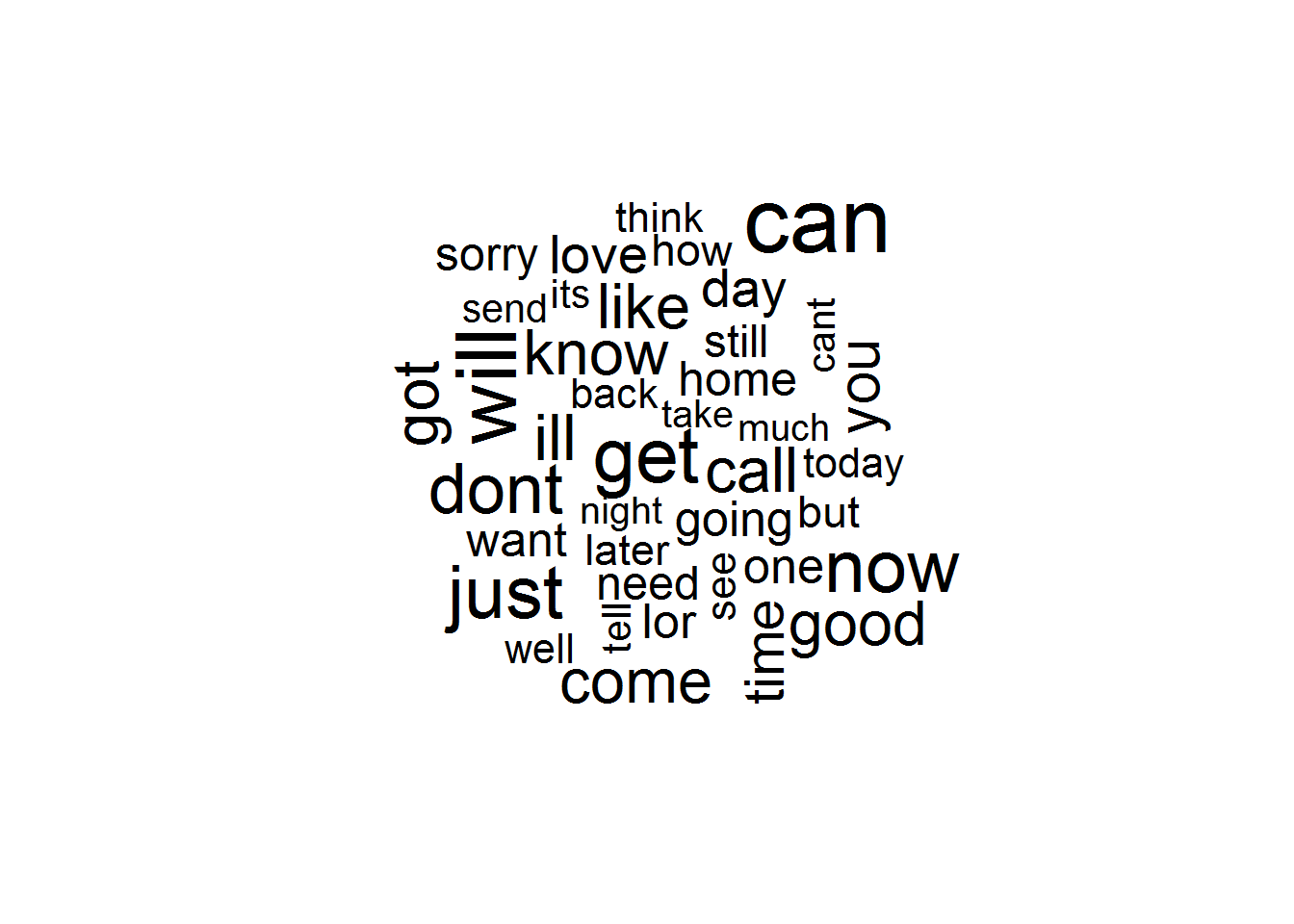
the ham cloud

Data preparation - creating indicator features for frequent words

Transform the sparse matrix into a data structure that can be used to train a naive Bayes classifier: we will eliminate any words that appear in less than five SMS messages, or less than about 0.1 percent of records in the training data.

Take a document term matrix and returns a character vector containing the words appearing at least a specified number of times.

sms_freq_words <- findFreqTerms(sms_dtm_train, 5)
str(sms_freq_words)

##  chr [1:1216] "â<U+0082>â<U+0080><U+009C>""| __truncated__ "abiola" "able" "abt" "accept" ...

Filter our DTM to include only the terms appearing in a specified vector.

sms_dtm_freq_train<- sms_dtm_train[ , sms_freq_words]
sms_dtm_freq_test <- sms_dtm_test[ , sms_freq_words]

The Naive Bayes classifier is typically trained on data with categorical features. This poses a problem, since the cells in the sparse matrix are numeric and measure the number of times a word appears in a message. We need to change this to a categorical variable that simply indicates yes or no depending on whether the word appears at all.

convert_counts <- function(x) {
x <- ifelse(x > 0, "Yes", "No")
}

# MARGIN = 1 is used for rows
sms_train <- apply(sms_dtm_freq_train, MARGIN = 2, convert_counts)
sms_test <- apply(sms_dtm_freq_test, MARGIN = 2, convert_counts)
str(sms_train)

##  chr [1:4169, 1:1216] "No" "No" "No" "No" "No" "No" "No" ...
##  - attr(*, "dimnames")=List of 2
##   ..$ Docs : chr [1:4169] "1" "2" "3" "4" ...
##   ..$ Terms: chr [1:1216] "â<U+0082>â<U+0080><U+009C>""| __truncated__ "abiola" "able" "abt" ...

str(sms_test)

##  chr [1:1390, 1:1216] "No" "No" "No" "No" "No" "No" "No" ...
##  - attr(*, "dimnames")=List of 2
##   ..$ Docs : chr [1:1390] "4170" "4171" "4172" "4173" ...
##   ..$ Terms: chr [1:1216] "â<U+0082>â<U+0080><U+009C>""| __truncated__ "abiola" "able" "abt" ...

Step 3 - training a model on the data

library(e1071) 

## Warning: package 'e1071' was built under R version 3.3.3

# build our model on the sms_train matrix
sms_classifier <- naiveBayes(sms_train, sms_train_labels)

The sms_classifier object now contains a naiveBayes classifier object that can be used to make predictions.

Step 4 - evaluating model performance

Recall that the unseen message features are stored in a matrix named sms_test, while the class labels (spam or ham) are stored in a vector named sms_test_labels

# use this classifier to generate predictions and then compare the predicted values to the true values.
sms_test_pred <- predict(sms_classifier, sms_test)

Compare the predictions to the true values. Add some additional parameters to eliminate unnecessary cell proportions and use the dnn parameter (dimension names) to relabel the rows and columns:

library(gmodels)

## Warning: package 'gmodels' was built under R version 3.3.3

CrossTable(sms_test_pred, sms_test_labels, prop.chisq = FALSE, prop.t = FALSE, dnn = c('predicted', 'actual'))

## 
##  
##    Cell Contents
## |-------------------------|
## |                       N |
## |           N / Row Total |
## |           N / Col Total |
## |-------------------------|
## 
##  
## Total Observations in Table:  1390 
## 
##  
##              | actual 
##    predicted |       ham |      spam | Row Total | 
## -------------|-----------|-----------|-----------|
##          ham |      1203 |        32 |      1235 | 
##              |     0.974 |     0.026 |     0.888 | 
##              |     0.997 |     0.175 |           | 
## -------------|-----------|-----------|-----------|
##         spam |         4 |       151 |       155 | 
##              |     0.026 |     0.974 |     0.112 | 
##              |     0.003 |     0.825 |           | 
## -------------|-----------|-----------|-----------|
## Column Total |      1207 |       183 |      1390 | 
##              |     0.868 |     0.132 |           | 
## -------------|-----------|-----------|-----------|
## 
## 

a total of only 4 + 32 = 36 of the 1,390 SMS messages were incorrectly classified (2.6 percent). - - - Among the errors were 4 out of 1,207 ham messages that were misidentified as spam, and 32 of the 183 spam messages were incorrectly labeled as ham.
The 4 legitimate messages that were incorrectly classified as spam could cause significant problems for the deployment of our filtering algorithm, because the filter could cause a person to miss an important text message. We should investigate to see whether we can slightly tweak the model to achieve better performance.

Step 5 - improving model performance

We didn’t set a value for the Laplace estimator while training our model. This allows words that appeared in zero spam or zero ham messages to have an indisputable say in the classification process. Just because the word “ringtone” only appeared in the spam messages in the training data, it does not mean that every message with this word should be classified as spam.

sms_classifier2 <- naiveBayes(sms_train, sms_train_labels, laplace = 1)
sms_test_pred2 <- predict(sms_classifier2, sms_test)
CrossTable(sms_test_pred2, sms_test_labels, prop.chisq = FALSE, prop.t = FALSE, prop.r = FALSE,
dnn = c('predicted', 'actual'))

## 
##  
##    Cell Contents
## |-------------------------|
## |                       N |
## |           N / Col Total |
## |-------------------------|
## 
##  
## Total Observations in Table:  1390 
## 
##  
##              | actual 
##    predicted |       ham |      spam | Row Total | 
## -------------|-----------|-----------|-----------|
##          ham |      1204 |        31 |      1235 | 
##              |     0.998 |     0.169 |           | 
## -------------|-----------|-----------|-----------|
##         spam |         3 |       152 |       155 | 
##              |     0.002 |     0.831 |           | 
## -------------|-----------|-----------|-----------|
## Column Total |      1207 |       183 |      1390 | 
##              |     0.868 |     0.132 |           | 
## -------------|-----------|-----------|-----------|
## 
## 

Adding the Laplace estimator reduced the number of false positives (ham messages erroneously classified as spam) from 4 to 3 and the number of false negatives from 32 to 31. Although this seems like a small change, it’s substantial considering that the model’s accuracy was already quite impressive

Summary

Naive Bayes constructs tables of probabilities that are used to estimate the likelihood that new examples belong to various classes. The probabilities are calculated using a formula known as Bayes’ theorem, which specifies how dependent events are related.
Although Bayes’ theorem can be computationally expensive, a simplified version that makes so-called “naive” assumptions about the independence of features is capable of handling extremely large datasets.
The Naive Bayes classifier is often used for text classification. To illustrate its effectiveness, we employed Naive Bayes on a classification task involving spam SMS messages. Preparing the text data for analysis required the use of specialized R packages for text processing and visualization.

Basic concepts of Bayesian methods

A study note from 'Machine Learning with R, 2nd edition'

What is Naive Bayes?

Case example:

The naive Bayes classification algorithm

The Laplace estimator

Case example 2

Solution

Using numeric features with naive Bayes

Solution

Example

Example - filtering mobile phone spam with the naive Bayes algorithm

Step 1 - collecting data

Step 2 - exploring and preparing the data

Data preparation - processing text data for analysis

Data preparation - splitting text documents into words

Data preparation - creating training and test datasets

Visualizing text data - word clouds

Data preparation - creating indicator features for frequent words

Step 3 - training a model on the data

Step 4 - evaluating model performance

Step 5 - improving model performance

Summary

CATALOG

FEATURED TAGS

FRIENDS